View the complete list of SEM features
SEM stands for structural equation modeling. SEM is a notation for specifying structural equations, a way of thinking about them, and methods for estimating their parameters.
SEM encompasses a broad array of models from linear regression to measurement models to simultaneous equations, including along the way confirmatory factor analysis (CFA), correlated uniqueness models, latent growth models, and multiple indicators and multiple causes (MIMIC).
Stata’s sem fits linear SEMs, and its features are described below. gsem provides extensions to linear SEMs that allow for generalized-linear models and multilevel models.
Use GUI or command language to specify model.
Standardized and unstandardized results.
Direct and indirect effects.
Goodness-of-fit statistics.
Tests for omitted paths and tests of model simplification including modification indices, score tests, and Wald tests.
Predicted values and factor scores.
Linear and nonlinear (1) tests of estimated parameters and (2) combinations of estimated parameters with CIs.
Estimation across groups is as easy as adding group(sex) to the command. Test for group invariance. Easily add or relax constraints across groups.
SEMs may be fitted using raw or summary statistics data.
Maximum likelihood (ML) and asymptotic distribution free (ADF) estimation. ADF is also known as generalized method of moments (GMM). Missing at random (MAR) data supported via FIML.
Robust estimate of standard errors and standard errors for clustered samples available.
Support for survey data including sampling weights, stratification and poststratification, and clustered sampling at one or more levels.
Enter your model graphically,
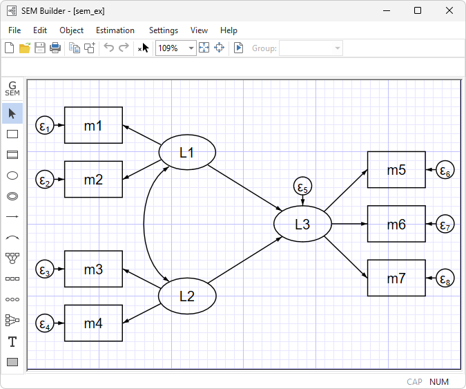
or use the command syntax
. sem (L1 -> m1 m2)
      (L2 -> m3 m4)
      (L3 <- L1 L2)
      (L3 -> m5 m6 m7)
It’s the same model either way.
Stata’s SEM Builder uses standard path notation.
In command syntax, you type the path diagram. Capitalized names are latent variables. Lowercased names are observed variables. You can type arrows in either direction. The above model could be equally well typed as
. sem (m1 m2 <- L1)
      (L2 -> m3 m4)
      (L3 <- L1 L2)
      (L3 -> m5 m6 m7)
and order does not matter, and neither does spacing:
. sem (m1 m2 <- L1) (L2 -> m3 m4) (L3 -> m5 m6 m7) (L3 <- L1 L2)
You can specify paths individually,
. sem (m1 <- L1) (m2 <- L1) (L2 -> m3) (L2 -> m4) (L3 -> m5) (L3 -> m6) (L3 -> m7) (L3 <- L1) (L3 <- L2)
or combined,
. sem (m1 m2 <- L1) (L2 -> m3 m4) (L3 -> m5 m6 m7) (L3 <- L1 L2)
Let’s fit a structural model with a measurement component using data from Wheaton, Muthén, Alwin, and Summers (1977):
. webuse sem_sm2, clear
(Structural model with measurement component)

. ssd describe

  Summary statistics data from https://www.stata-press.com/data/r17/sem_sm2.dta
  Observations:             932          Structural model with measurem..
     Variables:              13          25 May 2020 11:45
                                         (_dta has notes)
| Variable name Variable label |
| educ66 Education, 1966 occstat66 Occupational status, 1966 anomia66 Anomia, 1966 pwless66 Powerlessness, 1966 socdist66 Latin American social distance, 1966 occstat67 Occupational status, 1967 anomia67 Anomia, 1967 pwless67 Powerlessness, 1967 socdist67 Latin American social distance, 1967 occstat71 Occupational status, 1971 anomia71 Anomia, 1971 pwless71 Powerlessness, 1971 socdist71 Latin American social distance, 1971 |
Below we will demonstrate
Simplified versions of the model fit by the authors of the referenced paper appear in many SEM software manuals. One simplified model is

You can also readily fit this model using the following command:
. sem
   (anomia67 pwless67 <- Alien67)          /// measurement piece
   (anomia71 pwless71 <- Alien71)          /// measurement piece
   (Alien67 <- SES)                        /// structural piece
   (Alien71 <- Alien67 SES)                /// structural piece
   (    SES -> educ occstat66), nolog      /// measurement piece
And the results are
Endogenous variables
  Measurement: anomia67 pwless67 anomia71 pwless71 educ66 occstat66
  Latent:      Alien67 Alien71

Exogenous variables
  Latent: SES

Structural equation model                                  Number of obs = 932
Estimation method: ml

Log likelihood = -15246.469

 ( 1)  [anomia67]Alien67 = 1
 ( 2)  [anomia71]Alien71 = 1
 ( 3)  [educ66]SES = 1
| OIM | |||
| Coefficient std. err. z P>|z| [95% conf. interval] | |||
| Structural | |||
| Alien67 | |||
| SES | -.6140404 .0562407 -10.92 0.000 -.7242701 -.5038107 | ||
| Alien71 | |||
| Alien67 | .7046342 .0533512 13.21 0.000 .6000678 .8092007 | ||
| SES | -.1744153 .0542489 -3.22 0.001 -.2807413 -.0680894 | ||
| Measurement | |||
| anomia67 | |||
| Alien67 | 1 (constrained) | ||
| _cons | 13.61 .1126205 120.85 0.000 13.38927 13.83073 | ||
| pwless67 | |||
| Alien67 | .8884887 .0431565 20.59 0.000 .8039034 .9730739 | ||
| _cons | 14.67 .1001798 146.44 0.000 14.47365 14.86635 | ||
| anomia71 | |||
| Alien71 | 1 (constrained) | ||
| _cons | 14.13 .1158943 121.92 0.000 13.90285 14.35715 | ||
| pwless71 | |||
| Alien71 | .8486022 .0415205 20.44 0.000 .7672235 .9299808 | ||
| _cons | 14.9 .1034537 144.03 0.000 14.69723 15.10277 | ||
| educ66 | |||
| SES | 1 (constrained) | ||
| _cons | 10.9 .1014894 107.40 0.000 10.70108 11.09892 | ||
| occstat66 | |||
| SES | 5.331259 .4307503 12.38 0.000 4.487004 6.175514 | ||
| _cons | 37.49 .6947112 53.96 0.000 36.12839 38.85161 | ||
| var(e.anomia67) | 4.009921 .3582978 3.365724 4.777416 | ||
| var(e.pwless67) | 3.187468 .283374 2.677762 3.794197 | ||
| var(e.anomia71) | 3.695593 .3911512 3.003245 4.54755 | ||
| var(e.pwless71) | 3.621531 .3037908 3.072483 4.268693 | ||
| var(e.educ66) | 2.943819 .5002527 2.109908 4.107319 | ||
| var(e.occstat66) | 260.63 18.24572 227.2139 298.9605 | ||
| var(e.Alien67) | 5.301416 .483144 4.434225 6.338201 | ||
| var(e.Alien71) | 3.737286 .3881546 3.048951 4.581019 | ||
| var(SES) | 6.65587 .6409484 5.511067 8.038482 | ||
Notes:
Measurement component: In both 1967 and 1971 anomia and powerlessness are used to measure endogenous latent variables representing Alienation for the same two years. Education and occupational status are used to measure the exogenous latent variable SES.
Structural component: SES->Alien67 and SES->Alien71, and Alien67->Alien71.
The model vs. saturated chi-squared test indicates the model is a poor fit.
That the model is a poor fit leads us to looking at the modification indices:
. estat mindices

Modification indices
| Standard | |||
| MI df P>MI EPC EPC | |||
| Measurement | |||
| anomia67 | |||
| anomia71 | 51.977 1 0.00 .3906425 .4019984 | ||
| pwless71 | 32.517 1 0.00 -.2969297 -.2727609 | ||
| educ66 | 5.627 1 0.02 .0935048 .0842631 | ||
| pwless67 | |||
| anomia71 | 41.618 1 0.00 -.3106995 -.3594367 | ||
| pwless71 | 23.622 1 0.00 .2249714 .2323233 | ||
| educ66 | 6.441 1 0.01 -.0889042 -.0900664 | ||
| anomia71 | |||
| anomia67 | 58.768 1 0.00 .429437 .4173061 | ||
| pwless67 | 38.142 1 0.00 -.3873066 -.3347904 | ||
| pwless71 | |||
| anomia67 | 46.188 1 0.00 -.3308484 -.3601641 | ||
| pwless67 | 27.760 1 0.00 .2871709 .2780833 | ||
| educ66 | |||
| anomia67 | 4.415 1 0.04 .1055965 .1171781 | ||
| pwless67 | 6.816 1 0.01 -.1469371 -.1450411 | ||
| cov(e.anomia67,e.anomia71) | 63.786 1 0.00 1.951578 .5069627 | ||
| cov(e.anomia67,e.pwless71) | 49.892 1 0.00 -1.506704 -.3953794 | ||
| cov(e.anomia67,e.educ66) | 6.063 1 0.01 .5527612 .1608845 | ||
| cov(e.pwless67,e.anomia71) | 49.876 1 0.00 -1.534199 -.4470094 | ||
| cov(e.pwless67,e.pwless71) | 37.357 1 0.00 1.159123 .341162 | ||
| cov(e.pwless67,e.educ66) | 7.752 1 0.01 -.5557802 -.1814365 | ||
Notes:
There are lots of statistically significant paths we could add to the model.
Some of those statistically significant paths also make theoretical sense.
Two in particular that make sense are the covariances between e.anomia67 and e.anomia71, and between e.pwless67 and e.pwless71.
Let’s refit the model and include those two previously excluded covariances:
. sem
   (anomia67 pwless67 <- Alien67)          /// measurement piece
   (anomia71 pwless71 <- Alien71)          /// measurement piece
   (Alien67 <- SES)                        /// structural piece
   (Alien71 <- Alien67 SES)                /// structural piece
   (    SES -> educ occstat66)             /// measurement piece
          , cov(e.anomia67*e.anomia71)
          cov(e.pwless67*e.pwless71) nolog
And the results are
Endogenous variables
  Measurement: anomia67 pwless67 anomia71 pwless71 educ66 occstat66
  Latent:      Alien67 Alien71

Exogenous variables
  Latent: SES

Structural equation model                                  Number of obs = 932
Estimation method: ml

Log likelihood = -15213.046

 ( 1)  [anomia67]Alien67 = 1
 ( 2)  [anomia71]Alien71 = 1
 ( 3)  [educ66]SES = 1
| OIM | |||
| Coefficient std. err. z P>|z| [95% conf. interval] | |||
| Structural | |||
| Alien67 | |||
| SES | -.5752228 .057961 -9.92 0.000 -.6888244 -.4616213 | ||
| Alien71 | |||
| Alien67 | .606954 .0512305 11.85 0.000 .5065439 .707364 | ||
| SES | -.2270301 .0530773 -4.28 0.000 -.3310596 -.1230006 | ||
| Measurement | |||
| anomia67 | |||
| Alien67 | 1 (constrained) | ||
| _cons | 13.61 .1126143 120.85 0.000 13.38928 13.83072 | ||
| pwless67 | |||
| Alien67 | .9785952 .0619825 15.79 0.000 .8571117 1.100079 | ||
| _cons | 14.67 .1001814 146.43 0.000 14.47365 14.86635 | ||
| anomia71 | |||
| Alien71 | 1 (constrained) | ||
| _cons | 14.13 .1159036 121.91 0.000 13.90283 14.35717 | ||
| pwless71 | |||
| Alien71 | .9217508 .0597225 15.43 0.000 .8046968 1.038805 | ||
| _cons | 14.9 .1034517 144.03 0.000 14.69724 15.10276 | ||
| educ66 | |||
| SES | 1 (constrained) | ||
| _cons | 10.9 .1014894 107.40 0.000 10.70108 11.09892 | ||
| occstat66 | |||
| SES | 5.22132 .425595 12.27 0.000 4.387169 6.055471 | ||
| _cons | 37.49 .6947112 53.96 0.000 36.12839 38.85161 | ||
| var(e.anom~67) | 4.728874 .456299 3.914024 5.713365 | ||
| var(e.pwle~67) | 2.563413 .4060733 1.879225 3.4967 | ||
| var(e.anom~71) | 4.396081 .5171156 3.490904 5.535966 | ||
| var(e.pwle~71) | 3.072085 .4360333 2.326049 4.057398 | ||
| var(e.educ66) | 2.803674 .5115854 1.960691 4.009091 | ||
| var(e.occs~66) | 264.5311 18.22483 231.1177 302.7751 | ||
| var(e.Alien67) | 4.842059 .4622537 4.015771 5.838364 | ||
| var(e.Alien71) | 4.084249 .4038995 3.364613 4.957802 | ||
| var(SES) | 6.796014 .6524866 5.630283 8.203105 | ||
| cov(e.anom~67, | |||
| e.anomia71) | 1.622024 .3154267 5.14 0.000 1.003799 2.240249 | ||
| cov(e.pwle~67, | |||
| e.pwless71) | .3399961 .2627541 1.29 0.196 -.1749925 .8549847 | ||
Notes:
We find the covariance between e.anomia67 and e.anomia71 to be significant(Z=5.14).
We find the covariance between e.pwless67 and e.pwless71 to be insignificant at the 5% level (Z=1.29).


