Logistic regression

Stata supports all aspects of logistic regression. View the list of logistic regression features.

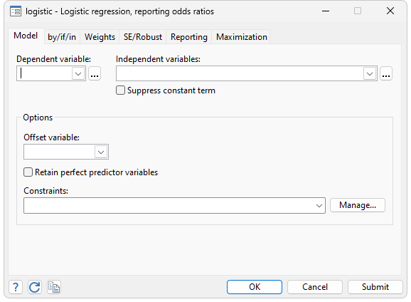
Stata’s logistic fits maximum-likelihood dichotomous logistic models:

. webuse lbw
(Hosmer & Lemeshow data)

. logistic low age lwt i.race smoke ptl ht ui

Logistic regression                                     Number of obs =    189
                                                        LR chi2(8)    =  33.22
                                                        Prob > chi2   = 0.0001
Log likelihood = -100.724                               Pseudo R2     = 0.1416




         low 
 
  Odds ratio   Std. err.      z    P>|z|     [95% conf. interval]

 
 
 

         age 
 
   .9732636   .0354759    -0.74   0.457     .9061578    1.045339

         lwt 
 
   .9849634   .0068217    -2.19   0.029     .9716834    .9984249

 
       
 

        race 
 

      Black  
 
   3.534767   1.860737     2.40   0.016     1.259736    9.918406

      Other  
 
   2.368079   1.039949     1.96   0.050     1.001356    5.600207

 
             
 

       smoke 
 
   2.517698    1.00916     2.30   0.021     1.147676    5.523162

         ptl 
 
   1.719161   .5952579     1.56   0.118     .8721455    3.388787

          ht 
 
   6.249602   4.322408     2.65   0.008     1.611152    24.24199

          ui 
 
     2.1351   .9808153     1.65   0.099     .8677528      5.2534

       _cons 
 
   1.586014   1.910496     0.38   0.702     .1496092     16.8134

Note: _cons estimates baseline odds.

The syntax of all estimation commands is the same: the name of the dependent variable is followed by the names of the independent variables. In this case, the dependent variable low (containing 1 if a newborn had a birthweight of less than 2500 grams and 0 otherwise) was modeled as a function of a number of explanatory variables. By default, logistic reports odds ratios; logit alternative will report coefficients if you prefer.

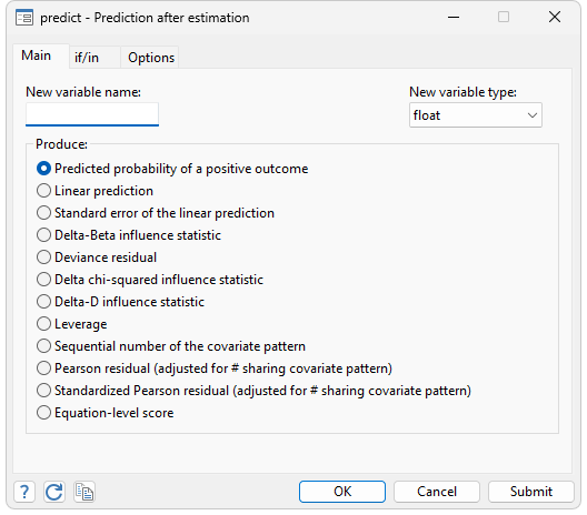
Once a model has been fitted, you can use Stata's predict to obtain the predicted probabilities of a positive outcome, the value of the logit index, or the standard error of the logit index. You can also obtain Pearson residuals, standardized Pearson residuals, leverage (the diagonal elements of the hat matrix), Delta chi-squared, Delta D, and Pregibon's Delta beta influence measures by typing a single command. All statistics are adjusted for the number of covariate patterns in the data—m-asymptotic rather than n-asymptotic in Hosmer and Lemeshow (2000) jargon. Every diagnostic graph suggested by Hosmer and Lemeshow can be drawn by Stata.

Also available are the goodness-of-fit test, using either cells defined by the covariate patterns or grouping, as suggested by Hosmer and Lemeshow; classification statistics and the classification table; and a graph and area under the ROC curve.

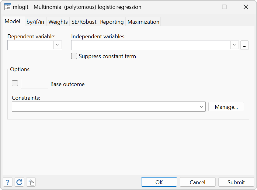
Stata’s mlogit performs maximum likelihood estimation of models with categorical dependent variables. It is intended for use when the dependent variable takes on more than two outcomes and the outcomes have no natural ordering. Uniquely, linear constraints on the coefficients can be specified both within and across equations using algebraic syntax. Much thought has gone into making mlogit truly usable. For instance, there are no artificial constraints placed on the nature of the dependent variable. The dependent variable is not required to take on integer, contiguous values such as 1, 2, and 3, although such a coding would be acceptable. Equally acceptable would be 1, 3, and 4, or even 1.2, 3.7, and 4.8.

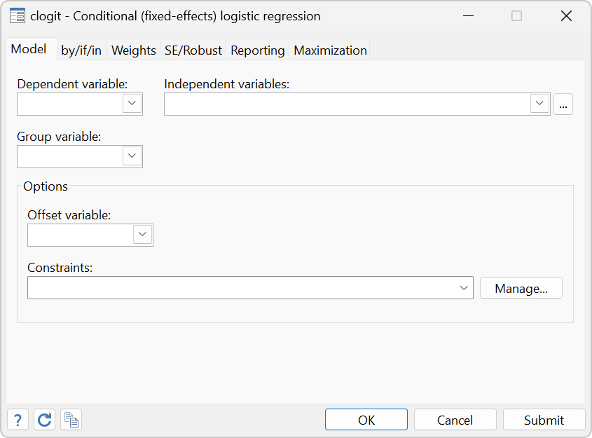
Stata’s clogit performs maximum likelihood estimation with a dichotomous dependent variable; conditional logistic analysis differs from regular logistic regression in that the data are stratified and the likelihoods are computed relative to each stratum. The form of the likelihood function is similar but not identical to that of multinomial logistic regression. Conditional logistic analysis is known in epidemiology circles as the matched case–control model and in econometrics as McFadden's choice model. The form of the data, as well as the nature of the sampling, differs across the two settings, but clogit handles both. clogit allows both 1:1 and 1:k matching, and there may even be more than one positive outcome per strata (which is handled using the exact solution).

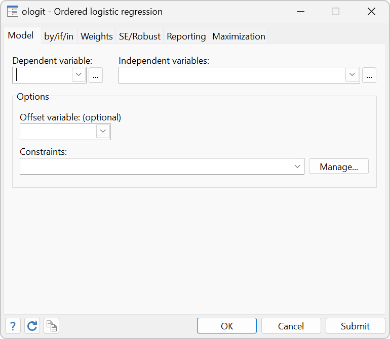
Stata’s ologit performs maximum likelihood estimation to fit models with an ordinal dependent variable, meaning a variable that is categorical and in which the categories can be ordered from low to high, such as “poor”, “good”, and “excellent”. Unlike mlogit, ologit can exploit the ordering in the estimation process. (Stata also provides oprobit for fitting ordered probit models.) As with mlogit the categorical dependent variable may take on any values whatsoever.

See Greene (2012) for a straightforward description of the models fitted by clogit, mlogit, ologit, and oprobit.