Introduction to structural equation modeling (SEM)

Do you know what SEM is? (If you know what SEM is, read an overview of Stata’s SEM capabilities.)

SEM stands for structural equation modeling. SEM is

1. A notation for specifying structural equation models.
2. A way of thinking about structural equation models.
3. Methods for estimating the parameters of structural equation models.

Stata’s sem command implements linear structural equation models.

For those of you unfamiliar with SEM, it is worth your time to learn about it if you ever fit linear regressions, multivariate linear regressions, seemingly unrelated regressions, or simultaneous systems, or if you are interested in generalized method of moments (GMM).

As you may have figured out, SEM is based on the linear model. What it brings to the table is flexible specification—nearly anything can be allowed to be correlated or constrained to be uncorrelated—and unobserved (latent) variables which can be treated (almost) as if they were observed.

SEM fits the first and second moments of the distribution of observed variables—means, variances, and covariances—rather than fitting the observed values themselves. Both maximum likelihood and GMM methods are available; sem uses a weighting matrix corresponding to asymptotic distribution free estimation in the SEM literature.

You still think of the model in the same way as usual, but in a model like

     yj = β0 + β1x1j + ... + βkxkj + ej

let’s now call e_j the error. Reserve the word residual for the true residuals of the SEMs, which are the differences between the observed and predicted moments.

When SEM is used to fit models that can be fit by the other linear estimators, results are the same, asymptotically the same—by which we mean different in finite samples, and there is no theoretical reason to prefer one set of estimated results to the other—or the SEM results are asymptotically the same and the SEM results should be better in finite samples because of theoretical reasons.

Notation

Individual structural equation models are usually described using path diagrams, such as

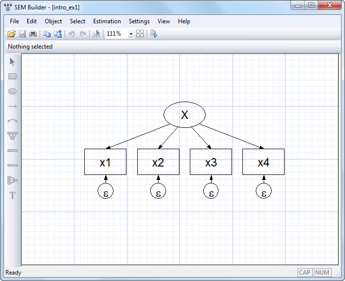
This diagram is composed of

1. Boxes and circles with variable names written inside them.
   1. Boxes contain variables that are observed in the data.
   2. Circles contain variables that are unobserved, known as latent variables.
2. Arrows, called paths, that connect some of the boxes and circles.
   1. When a path points from one variable to another, that means the first variable affects the second.
   2. More precisely, if s->d, that means to add β_k to the linear equation for d. β_k is called the path coefficient.
   3. Sometimes small numbers are written along the arrow connecting two variables. That means β_k is constrained to be the value specified.
   4. When no number is written along the arrow, the corresponding coefficient is to be estimated from the data. Sometimes symbols are written along the path arrow to emphasize this, and sometimes not.
   5. The same path diagram used to describe the model can be used to display the results of estimation. In that case, estimated coefficients appear along the paths.
3. Not shown above are curved, double-headed paths that are used to indicate covariances where they would not be otherwise assumed. Exogenous variables are assumed to be correlated.

Thus the above figure corresponds to the equations

     x1 = α1 + β1X + e.x1

     x2 = α2 + β2X + e.x2

     x3 = α3 + β3X + e.x3

     x4 = α4 + β4X + e.x4

There’s a third way of writing this model, namely

     (x1<-X) (x2<-X) (x3<-X) (x4<-X)

This is the way we could write the model if we wanted to use sem’s command syntax rather than drawing the model in sem’s GUI. The full command we would type would be

     . sem (x1<-X) (x2<-X) (x3<-X) (x4<-X)

However we write this model, what is it? It is a measurement model, a term loaded with meaning for some researchers. X might be mathematical ability. x1, x2, x3, and x4 might be scores from tests designed to measure mathematical ability. x1 might be the score based on your answers to a series of questions after reading this section.

The model we have just drawn, written in mathematical notation, or written in Stata command notation can be interpreted in other ways too. Look at this diagram:

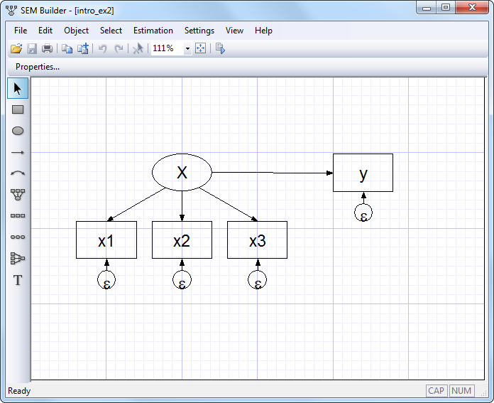
Despite appearances, this diagram is identical to the previous diagram except that we have renamed x4 to be y. The fact that we changed a name obviously does not matter substantively. That fact that we have rearranged the boxes in the diagram is irrelevant, too; paths connect the same variables in the same directions. The equations for the above diagrams are the same as the previous equations with the substitution of y for x4:

     x1 = α1 + β1X + e.x1

     x2 = α2 + β2X + e.x2

     x3 = α3 + β3X + e.x3

     y = α4 + β4X + e.y

The Stata command notation changes similarly,

     (x1<-X) (x2<-X) (x3<-X) (y<-X)

Many people looking at the model written in this way might decide that it is not a measurement model but a measurement error model. y depends on X, but we do not observe X. We do observe x1, x2, and x3, each a measurement of X but with error. Our interest is in knowing β₄, the effect of true X on y.

A few others might disagree and instead see a model for interrater agreement. Obviously we have four raters who each make a judgment, and we want to know how well the judgment process works and how well each of these raters perform.

Measurement error with SEM

You are now ready to return to our description of Stata’s new sem command, but before you do, let us show you an example we think will appeal to you.

In our documentation, we have an example of a single-factor measurement model, which is demonstrated using the following data:

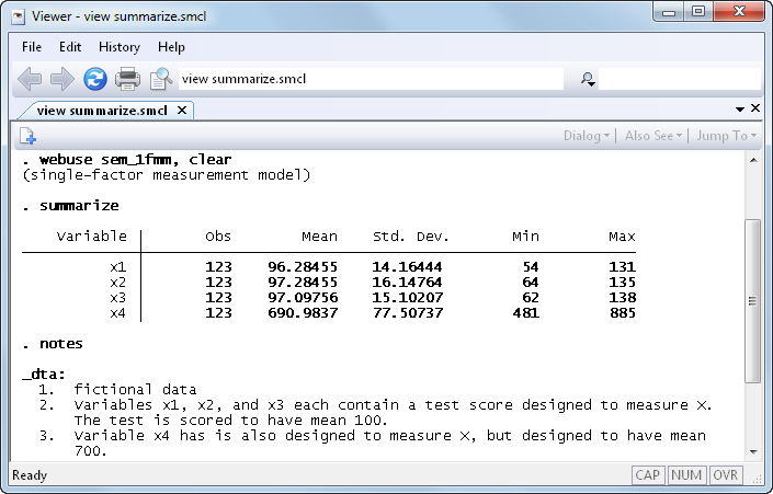
As we mentioned above, if we rename variable x4 to be y, we can reinterpret this measurement model as a measurement error model. In this interpretation, X is the unobserved true value. x1, x2, and x3 are each measurements of X, but with error. Meanwhile, y (x4) is really something else entirely. Perhaps y is earnings, and we believe

     y = α4 + β4X + e.y

We are interested in β₄, the effect of true X on y.

If we were to go back to the data and type regress y x1, we would obtain an estimate of β₄, but we would expect that estimate to be biased toward zero because of the errors-in-variable problem. The same applies for y on x2 and y on x3. If we do that, we obtain

     β4 based on regress y x1      4.09
     β4 based on regress y x2      3.71
     β4 based on regress y x3      3.70

In the example in our manual, we fit

     . sem (x1<-X) (x2<-X) (x3<-X) (y<-X)

and we obtained

     β4 based on sem (y<-X)      6.89

That β₄ might be 6.89 seems plausible because we expect the estimate to be larger than the estimates we obtain using the variables measured with error. In fact, we can tell you that the 6.89 estimate is quite good because we at StataCorp know that the true value of β₄ is 7.

Now you can return to our description of Stata’s structural equation modeling (SEM) features.

Back to highlights