Receiver operating characteristics (ROC)

You can now model ROC curves that control for covariates. Think of it like regression for ROC.

Norton et al. (2000) examined a neonatal audiology study on hearing impairment. A hearing test was applied to children aged 30 to 53 months. It is believed that the classifier y1 (DPOAE 65 at 2kHz) becomes more accurate at older ages.

In Stata 12, we can use rocreg with these data to model how sensitivity and specificity of this test depends on age. The extra effect of current age on y1 when the child has hearing impairment is estimated by specifying roccov(). The control population effect of current age and gender of the child is estimated by specifying ctrlcov().

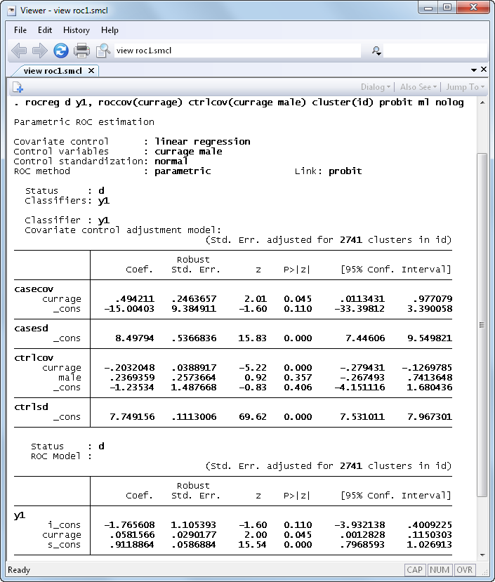
The results show us that current age has a borderline significant positive effect on the ROC curve (p-value = 0.045).

We can use the new command rocregplot to compare ROC at various ages. We will draw the curve for ages of 50 and 40 months and add some graph options to make the legend pretty and place it inside the graph.

rocregplot, at1(currage=40) at2(currage=50) ///
legend(order(3 "reference" 1 "40 mos." 2 "50 mos.") ring(0) rows(3) pos(5)) ///
title("ROC, by age") xsize(4) ysize(4)

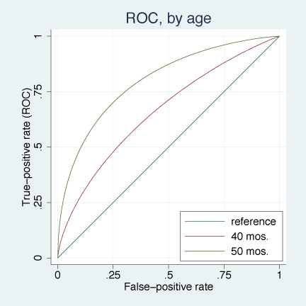
Area under the curve (AUC) increases with age.

We could also test whether AUC increases with age, estimate sensitivity for a given specificity (and vice versa), and estimate partial AUC (area to a given point of false positive), all controling for age.

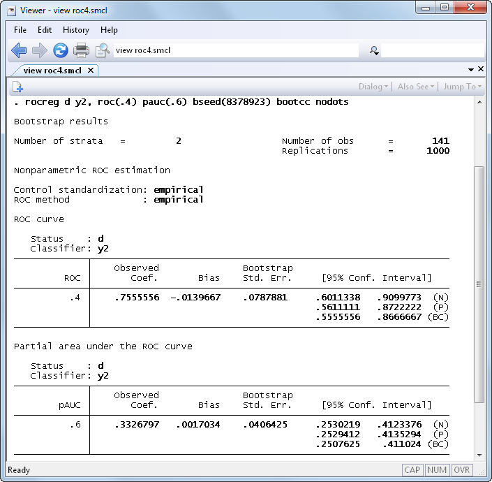
Wieand et. al. (1989) examined a pancreatic cancer study. No covariates were recorded, and the study was a case–control study.

We use rocreg to estimate the ROC curve for the classifier y2 (CA 125) that was examined. A nonparametric estimate is used, and we bootstrap to obtain standard errors. We estimate the sensitivity for the specificity value of .6 through the roc() option, which takes argument 1-specificity. The partial area under the curve (pAUC), the area under the ROC curve up to a given 1-specificity value, is estimated for the specificity of .4 with the pauc() option. The case–control sampling of the study is indicated to rocreg via the bootcc option.

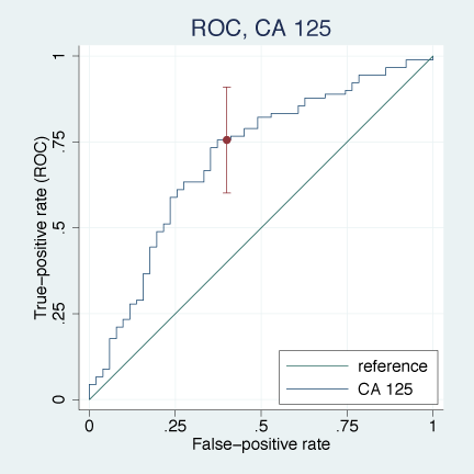
We can use rocregplot to see the ROC curve for y2 (CA 125). We also ask for normal-based confidence band for ROC value at the specificity of .6.

rocregplot, plot1opts(msymbol(i)) ///
legend(order(2 "reference" 1 "CA 125") ring(0) rows(2) pos(5)) ///
xsize(4) ysize(4) title("ROC, CA 125")

Back to highlights

References

Norton, S. J., M. P. Gorga, J. E. Widen, R. C. Folsom, Y. Sininger B. Cone-Wesson, B. R. Vohr, K. Mascher, and K. Fletcher. 2000.

Identification of neonatal hearing impairment: Evaluation of transient evoked otoacoustic emission, distortion product otoacoustic emission, and auditory brain stem response test performance. Ear and Hearing 21: 508–528.

Wieand, S., M. H. Gail, B. R. James, and K. L. James. 1989.

A family of nonparametric statistics for comparing diagnostic markers with paired or unpaired data. Biometrika 76: 585–592.

Pepe, M. S. 2003.

The Statistical Evaluation of Medical Tests for Classification and Prediction. New York: Oxford University Press.

See New in Stata 12 for more about what was added in Stata Release 12.