This page contains only historical information and is not about the current release of Stata. Please see our Stata 11 page for information on the current version of Stata.

Survival statistics

1. Existing estimation commands stcox and streg may now be used with the svy: prefix and so can fit models for complex survey data; see [ST] stcox and [ST] streg.
2. New command stpower provides sample-size and power calculations for survival studies that use Cox proportional hazards regressions, log-rank tests for two groups, or differences in exponentially distributed hazards or log hazards.
   
   
   1. stpower cox estimates required sample size (given power) or power (given sample size) or the minimal detectable coefficient (given power and sample size) for models with multiple covariates. The command provides options to account for possible correlation between the covariate of interest and other predictors and for withdrawal of subjects from the study. See [ST] stpower cox.
   2. stpower logrank estimates required sample size (given power) or power (given sample size) or the minimal detectable hazard ratio (given power and sample size) for studies comparing survivor functions of two groups by using the log-rank test. Both the Freedman (1982) and the Schoenfeld (1981) methods are provided. The command allows for unequal allocation of subjects between the groups and possible withdrawal of subjects. Estimates can be adjusted for uniform accrual. See [ST] stpower logrank.
   3. stpower exponential estimates sample size (given power) or power (given sample size) of tests of the difference between hazards or log hazards of two groups under the assumption of exponential survivor functions (also known as the exponential test). Both the Lachin–Foulkes and Rubinstein–Gail–Santner methods are provided. Unequal group allocation, uniform or truncated exponential accrual, and different exponential losses due to follow-up in each group are allowed. See [ST] stpower exponential.
   The stpower commands allow automated production of customizable tables and have options to assist with creating graphs of power curves. See [ST] stpower.
3. Concerning existing command sts graph,
   
   
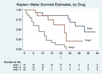
   1. New option risktable() places a subjects-at-risk table underneath and aligned to the survival or hazard plot.
   2. New option ci replaces old options gwood, cna, and cihazard. sts graph will choose the appropriate confidence interval on the basis of the function being graphed.
   3. Confidence intervals are now graphed using shaded areas, and new options plotopts() and ciopts() allow you to control how plots and confidence intervals look.
   4. New option censopts() controls the appearance of ticks and markers produced by existing option censored().
   5. Boundary computations for smoothing hazards have been improved. New option noboundary specifies that no boundary correction be done.
   6. The lower bound of the range to plot the hazard function now extends to zero.
   7. Option na has been renamed cumhaz. na may still be used.
   See [ST] sts graph. Setting version to less than 10 restores previous behavior.
4. For sts list, option na has been renamed cumhaz. na may be used as a synonym for cumhaz. See [ST] sts list.
5. Improvements to stcurve analogous to those of sts graph have been made.
   
   
   1. Boundary computations for smoothing hazards have been improved. New option noboundary specifies that no boundary correction be done.
   2. The lower bound of the range to plot the hazard function now extends to zero.
   See [ST] stcurve.
6. All st estimation commands accept option vce(vcetype). As mentioned in More new statistical features, vce(robust) and vce(cluster varname) are the right ways to specify the old robust and cluster() options, and vce() now allows other VCE calculations as well.
7. Existing command predict after stcox has a new option, scores, that allows generating variables with the partial coefficient score residuals; see [ST] stcox postestimation.
8. Existing command ltable has new options byopts(), plot#opts(), and ci#opts() that allow for more customization of the graph. New option ci adds confidence intervals to the graph. See [ST] ltable.
9. Existing command stphplot has a new option plot#opts() that allows for most customizations of the graph. See [ST] stcox diagnostics.
10. Existing command stcoxkm has new options byopts(), obsopts(), obs#opts(), predopts(), and pred#opts() that allow for most customizations of the graph. See [ST] stcox diagnostics.
11. Existing command cc has new option tarone that produces Tarone’s (1985) adjustment of the Breslow–Day test for homogeneity test of odds ratios. See [ST] epitab.
12. Existing command stdes has been renamed to stdescribe. stdes continues to work. See [ST] stdescribe.
13. The [ST] manual has an expanded glossary.

Back to highlights