1 item has been added to your cart.

Endogenous variables

Stata’s new ivregress command allows you to fit linear equations with endogenous regressors by the generalized method of moments (GMM) and limited-information maximum likelihood (LIML), as well as two-stage least squares (2SLS).

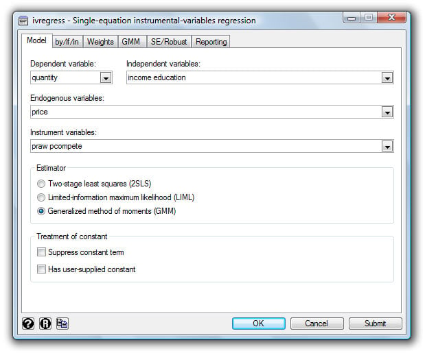
To fit a model of quantity consumed on income, education level, and price by using the heteroskedasticity-robust GMM estimator, with the prices of raw materials and a competing product as additional instruments, you fill in the dialog like this:

or type

. ivregress gmm quantity income education (price = praw pcompete)

To use the LIML estimator instead, you just click the box that says LIML on the dialog box or change gmm to liml.

ivregress can provide robust, cluster robust, jackknife, bootstrap, and heteroskedasticity- and autocorrelation-consistent (HAC) standard errors. With HAC standard errors you can select the Bartlett, Parzen, or quadratic spectral kernel, and you can specify the number of lags or request that Newey and West’s optimal lag-selection algorithm be used. The GMM estimator allows you to choose among robust, cluster robust, and HAC weight matrices.

After estimation with ivregress, you can use

• estat firststage to obtain various statistics measuring the relevance of instrumental variable’s. First-stage R², partial R², F statistics, Shea’s partial R², and the Cragg and Donald minimum eigenvalue statistic, along with Stock and Yogo’s critical values for tests of weak instruments, are available.
• estat overid provides tests of overidentifying restrictions. For the 2SLS estimator, Sargan’s and Basmann’s chi-squared tests are available, as is Wooldridge’s robust score test. After LIML estimation, the Anderson–Rubin chi-squared test and Basmann’s F test are available, and after GMM estimation, Hansen’s J statistic is available.

Example

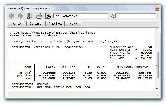
Is the cost to rent an apartment related to the price of houses in a community? With state-level data on hand, we believe that the rental rate is a linear function of housing prices and the percentage of a state’s population living in urban areas. However, we suspect that random shocks that affect rental rates also affect housing prices, so we treat the housing price variable hsngval as endogenous. We have median family income data along with regional dummies that can be used as additional instruments.

Let’s fit our model by using the LIML estimator. In Stata, we type

. use http://www.stata-press.com/data/r10/hsng2

. ivregress liml rent pcturban (hsngval = faminc reg2-reg4)

Before we dwell on these results, we should first check to make sure that the instruments are sufficiently correlated with hsngval. We can do that by using estat firststage:

. estat firststage

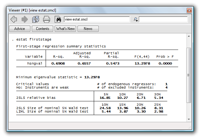
All of the R² statistics are relatively high, so they do not imply a weak-instrument problem. The F statistic is above the often-used threshold of 10. Since we are using the LIML estimator, we look at the final line of critical values in the second table. Suppose that we are willing to accept at most a rejection rate of 10% of a nominal 5% Wald test. Here we can reject the null hypothesis that the instruments are weak, since the test statistic of 13.30 exceeds its critical value of 5.44. On the basis of this test, we do not have a weak-instrument problem. Because our model has only one endogenous regressor, the minimum eigenvalue statistic is equal to the F statistic reported in the first table.

We should also do a test of overidentifying restrictions to verify the validity of our excluded instruments. estat overid makes that easy:

. estat overid

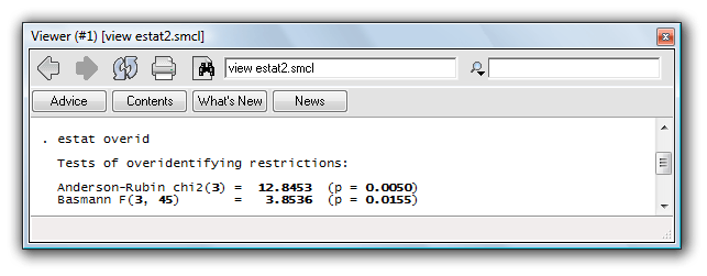
Here we reject the null hypothesis that our instruments are valid. If we were to pursue this model further, we would probably reconsider whether not including faminc as a regressor made sense. Families with higher incomes probably demand larger, more expensive apartments. These tests also assume that the errors are independently and identically distributed. Heteroskedasticity could be affecting these results as well. After fitting a model with the 2SLS estimator, estat overid can perform a test of overidentifying restrictions that is robust to heteroskedasticity.

Back to highlights