1 item has been added to your cart.

Choice modeling

1. New command asclogit performs alternative-specific conditional logit regression, including McFadden’s choice model. For models whose regressors vary by alternative instead of by case, asclogit is more convenient than clogit.
2. New command asroprobit performs alternative-specific rank-ordered probit regression, allowing you to model alternative-specific effects and the covariance structure of the alternatives.
3. New command exlogistic performs exact logistic regression. For more information, click here.
4. Stata’s conditional logit command clogit now works with survey data.
5. Stata’s nlogit command for nested logit has been rewritten and has a new, better syntax and runs faster; it now fits a model consistent with random utility maximization by default. The new nlogit now allows unbalanced groups and allows groups to have different sets of alternatives. Let us show you:




. use http://www.stata-press.com/data/r10/restaurant, clear

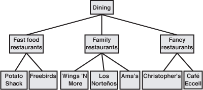
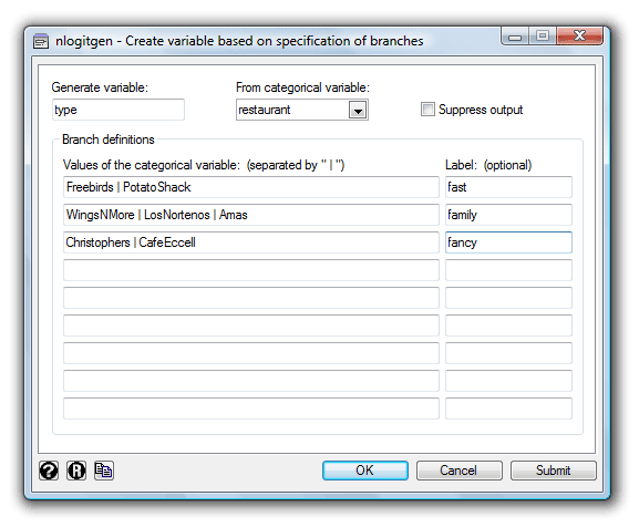
. nlogitgen type = restaurant(fast:Freebirds | PotatoShack,  
     family: WingsNmore | LosNortenos | Amas, 
     fancy: Christophers | CafeEccell) 

    new variable type is generated with 3 groups
    label list lb_type
    lb_type:
               1 fast
               2 family
               3 fancy

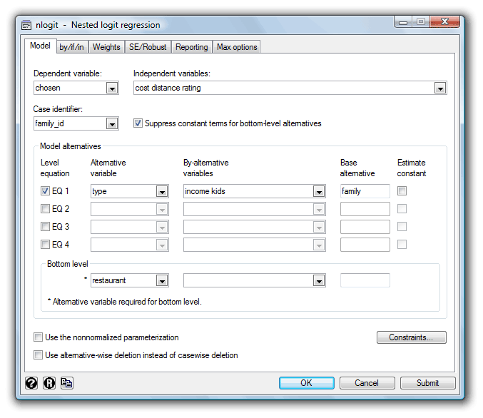
. nlogit chosen cost distance rating || type: income kids, 
     base(family) || restaurant:, noconst case(family_id)

    tree structure specified for the nested logit model

     type    N      restaurant    N   k 
    -------------------------------------
     fast   600 --- Freebirds    300  12
                 +- PotatoShack  300  15
     family 900 --- Amas         300  78
                 |- LosNortenos  300  75
                 +- WingsNmore   300  69
     fancy  600 --- Christophers 300  27
                 +- CafeEccell   300  24
    -------------------------------------
                         total  2100 300

    k = number of times alternative is chosen
    N = number of observations at each level

    Iteration 0:   log likelihood = -541.93581  
    Iteration 1:   log likelihood = -517.95909  (backed up)
    Iteration 2:   log likelihood = -511.99261  (backed up)
      (output omitted)
    Iteration 16:  log likelihood = -485.47333  
    Iteration 17:  log likelihood = -485.47331  

    RUM-consistent nested logit regression         Number of obs      =       2100
    Case variable: family_id                       Number of cases    =        300

    Alternative variable: restaurant               Alts per case: min =          7
                                                                  avg =        7.0
                                                                  max =          7

                                                      Wald chi2(7)    =      46.71
    Log likelihood = -485.47331                       Prob > chi2     =     0.0000

    ------------------------------------------------------------------------------
          chosen |      Coef.   Std. Err.      z    P>|z|     [95% Conf. Interval]
    -------------+----------------------------------------------------------------
    restaurant   |
            cost |  -.1843847   .0933975    -1.97   0.048    -.3674404   -.0013289
        distance |  -.3797474   .1003828    -3.78   0.000    -.5764941   -.1830007
          rating |    .463694   .3264935     1.42   0.156    -.1762215     1.10361
    ------------------------------------------------------------------------------
    type equations
    ------------------------------------------------------------------------------
    fast         |
          income |  -.0266038   .0117306    -2.27   0.023    -.0495952   -.0036123
            kids |  -.0872584   .1385026    -0.63   0.529    -.3587184    .1842016
    -------------+----------------------------------------------------------------
    family       |
          income |     (base)
            kids |     (base)
    -------------+----------------------------------------------------------------
    fancy        |
          income |   .0461827   .0090936     5.08   0.000     .0283595    .0640059
            kids |  -.3959413   .1220356    -3.24   0.001    -.6351267   -.1567559
    ------------------------------------------------------------------------------
    dissimilarity parameters
    ------------------------------------------------------------------------------
    type         |           
       /fast_tau |   1.712878    1.48685                     -1.201295    4.627051
     /family_tau |   2.505113   .9646351                       .614463    4.395763
      /fancy_tau |   4.099844   2.810123                     -1.407896    9.607583
    ------------------------------------------------------------------------------
    LR test for IIA (tau = 1):           chi2(3) =     6.87   Prob > chi2 = 0.0762
    ------------------------------------------------------------------------------

Here’s a complete list of what’s new in choice modeling:

1. New estimation command asclogit performs alternative-specific conditional logistic regression, which includes McFadden’s choice model. Postestimation command estat alternatives reports alternative-specific summary statistics. estat mfx reports marginal effects of regressors on probabilities of each alternative. See [R] asclogit and [R] asclogit postestimation.
2. New estimation command asroprobit performs alternative-specific rank-ordered probit regression. asroprobit is related to rank-ordered logistic regression (rologit) but allows modeling alternative-specific effects and modeling the covariance structure of the alternatives. Postestimation command estat alternatives provides summary statistics about the alternatives in the estimation sample. estat covariance displays the variance–covariance matrix of the alternatives. estat correlation displays the correlation matrix of the alternatives. estat mfx computes the marginal effects of regressors on the probability of the alternatives. See [R] asroprobit and [R] asroprobit postestimation.
3. Stata now has exact logistic and exact Poisson regression. Rather than having their inference based on asymptotic normality, exact estimators enumerate the conditional distribution of the sufficient statistics and then base inference upon that distribution. In small samples, exact methods have better coverage than asymptotic methods, and exact methods are the only way to obtain point estimates, tests, and confidence intervals from covariates that perfectly predict the observed outcome.
   
   Postestimation command estat se reports odds ratios and their asymptotic standard errors. estat predict, available only after exlogistic computes predicted probabilities, asymptotic standard errors, and exact confidence intervals for single cases.
   
   See [R] exlogistic and [R] expoisson.
4. Existing estimation command nlogit was rewritten and has new, better syntax and runs faster when there are more than two levels. Old syntax is available under version control. nlogit now optionally fits the random utilities maximization (RUM) model as well as the nonnormalized model that was available previously. The new nlogit now allows unbalanced groups and allows groups to have different sets of alternatives. nlogit now excludes entire choice sets (cases) if any alternative (observation) has a missing value; use new option altwise to exclude just the alternatives (observations) with missing values. Finally, vce(robust) is allowed regardless of the number of nesting levels. See [R] nlogit.
5. Existing estimation command asmprobit has the following enhancements:
   
   
   1. The new default parameterization estimates the covariance of the alternatives differenced from the base alternative, making the estimates invariant to the choice of base. New option structural specifies that the previously structural (nondifferenced) covariance parameterization be used.
   2. asmprobit now permits estimation of the constant-only model.
   3. asmprobit now excludes entire choice sets (cases) if any alternative (observation) has a missing value; use new option altwise to exclude just the alternatives (observations) with missing values.
   4. New postestimation command estat mfx computes marginal effects after asmprobit.
   See [R] asmprobit and [R] asmprobit postestimation.
6. Existing estimation command clogit now accepts pweights and may be used with the svy: prefix.
   
   Also, clogit used to be willing to produce cluster-robust VCEs when the groups were not nested within the clusters. Sometimes, this VCE was consistent, and other times it was not. You must now specify the new nonest option to obtain a cluster-robust VCE when the groups are not nested within panels.
   
   predict after clogit now accepts options that calculate the Δβ influence statistic, the Δchi² lack-of-fit statistic, the Hosmer and Lemeshow leverage, the Pearson residuals, and the standardized Pearson residuals.
   
   See [R] clogit and [R] clogit postestimation.
7. Existing estimation command mprobit now allows pweights, may now be used with the svy: prefix, and has new option probitparam that specifies that the probit variance parameterization, which fixes the variance of the differenced latent errors between the scale and the base alternatives to one, be used. See [R] mprobit.
8. Existing estimation command rologit now allows vce(bootstrap) and vce(jackknife). See [R] rologit.

Back to highlights