

In the spotlight: Bayesian IRT–4PL model
Item response theory (IRT) is often used for modeling the relationship between the latent abilities of a group of subjects and the examination items used for measuring their abilities. Stata 14 introduced a suite of commands for fitting IRT models using maximum likelihood; see, for example, "In the spotlight: irt" by Rafal Raciborski in Stata News, Volume 30 Number 3 and the [IRT] Item Response Theory Reference Manual for more details. One-parameter logistic (1PL), 2PL, and 3PL IRT models are commonly used to model binary responses. Models beyond 3PL, such as 4PL and 5PL models, have not been as widely used. One of the reasons is the difficulty in estimating the additional parameters introduced by these models using maximum likelihood. In recent years, these models have been reconsidered within the Bayesian framework (Loken and Rulison 2010; Fox 2010; Kim and Bolt 2007). In this article, we demonstrate how to fit a Bayesian 4PL model using bayesmh.
Data
We will use the abridged version of the mathematics and science data from DeBoeck and Wilson (2004), which contains 800 student responses, y, to 9 test questions (items) intended to measure mathematical ability. To fit IRT models using bayesmh, the data must be in long form with items, item, recorded as multiple observations per subject, id.
Model
We consider the following 4PL model,
P(Yij = 1) = c + (d–c)InvLogit{ai(θj–bi)}, c < d < 1
where i = 1, 2, ..., 9 and j = 1, 2, ..., 800. The 4PL model extends the 3PL model by adding an upper asymptote parameter d ≠ 1. The d parameter can be viewed as an upper limit on the probability of correct response to the ith item. The probability of giving correct answers by subjects with very high ability can thus be no greater than d. ai and bi are item-specific discrimination and difficulties. Here we consider a common guessing parameter c and a common upper asymptote parameter d, but they can also be item specific. InvLogit() is an inverse-logit function. The latent abilities θj are assumed to be normally distributed:
θj ∼ N(0,1)
A Bayesian formulation also requires prior specifications for all other model parameters. This is an important step in Bayesian modeling and must be considered carefully. For illustration, we consider the following priors.
Discrimination parameters ai's are assumed to be positive and are often modeled in the log scale. Because we have no prior knowledge about the discrimination and difficulty parameters, we assume that the prior distributions of ln(ai) and bi have support on the whole real line and are symmetric. A normal prior distribution is thus a natural choice. To control the impact of the prior on these parameters, we consider a hierarchical Bayesian model specification and introduce hyperparameters to model means and variances of the normal prior distribution.
ln(ai) ∼ N(μa,σ2a)
bi ∼ N(μb,σ2b)
We use informative priors for the guessing parameter c and the upper asymptote parameter d. We assume that the prior mean of c is about 0.1 and use an inverse-gamma prior with shape 10 and scale 1 for c. We restrict d to the (0.8,1) range and assign it a Uniform(0.8,1) prior.
c ∼ InvGamma(10,1)
d ∼ Uniform(0.8,1)
The mean hyperparameters, μa and μb, and variance hyperparameters, σ2a and σ2b, require informative prior specifications. We assume that the means are centered at 0 with a variation of 0.1. To lower the variability of the ln(ai) and bi parameters, we use an inverse-gamma prior with shape 10 and scale 1 for the variance parameters so that their prior means are about 0.1.
μa,μb ∼ N(0,0.1)
σ2a,σ2b ∼ InvGamma(10,1)
Using bayesmh
We specify the model above using bayesmh as follows:
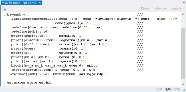
The first two lines model the probability of success of a Bernoulli outcome as a nonlinear function of model parameters. Subject-specific parameters {subj:} and item-specific parameters {discrim:} and {diff:} are included as "random effects" in the model by using the corresponding redefine() options (available in Stata 14.1) for computational efficiency. The priors for model parameters are specified in the corresponding prior() options. We place model parameters in separate blocks to improve the simulation efficiency and provide more sensible initial values for some of the parameters. Here we treat the abilities {subj:i.id} as nuisance parameters and exclude them from the final results. We use a longer burn-in period, burnin(5000), to allow for longer adaptation of the MCMC sampler, which is needed given the large number of parameters in the model.
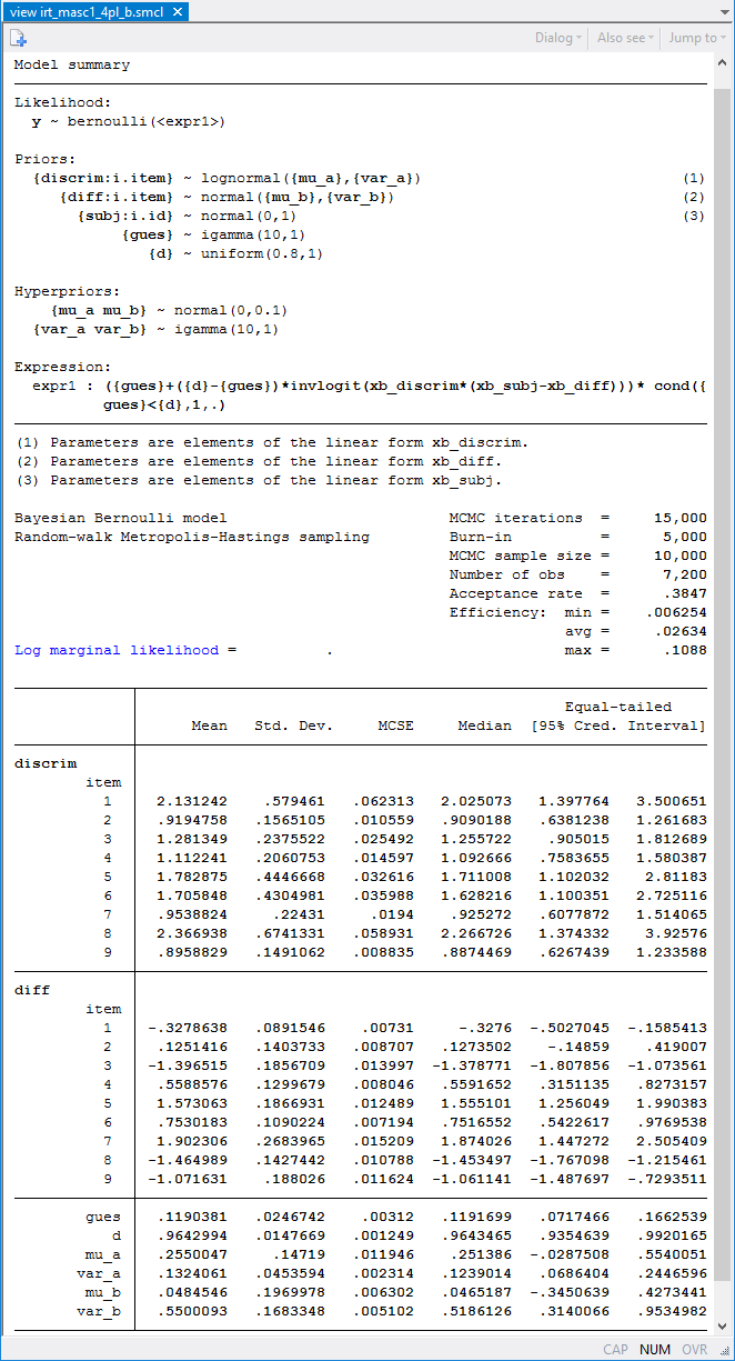
bayesmh produces the following results:
The upper asymptote parameter d is estimated to be 0.96 with a 95% credible interval of [0.94, 0.99]. The estimate is fairly close to one, so a simpler 3PL model may be sufficient for these data.
Comparing models
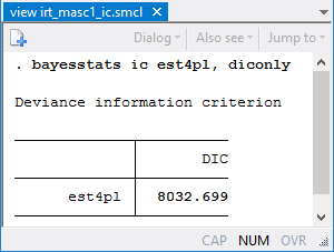
More formally, we can compare deviance information criteria (DIC) of the 4PL and the 3PL (with d = 1) models.
The DIC of the 3PL model (not shown here) is 8049.4. The 4PL model has a lower DIC value, 8032.7, which suggests that the 4PL model provides a better fit. However, we should not rely solely on the DIC values to make our final model selection. A practitioner may still prefer the simpler 3PL model given that the upper asymptote estimate is close to one.
For more examples of Bayesian binary IRT models and details about model specifications, see our blog entry: "Bayesian binary item response theory models using bayesmh.
—Nikolay Balov
Senior Statistician and Software Developer, StataCorp
—Yulia Marchenko
Executive Director of Statistics, StataCorp
References
De Boeck, P., and M. Wilson, ed. 2004. Explanatory Item Response Models: A Generalized Linear and Nonlinear Approach. New York: Springer.
Fox, J.-P. 2010. Bayesian Item Response Modeling: Theory and Applications. New York: Springer.
Kim, J.-S., and D. M. Bolt. 2007. Estimating item response theory models using Markov chain Monte Carlo methods. Educational Measurement: Issues and Practice 26: 38–51.
Loken, E., and K. L. Rulison. 2010. Estimation of a four-parameter item response theory model. British Journal of Mathematical and Statistical Psychology 63: 509–525.


