1 item has been added to your cart.

How do I graph data onto a map with spmap?

Introduction

With spmap, you can graph data onto maps and produce results such as these:

spmap is a community-contributed command by Maurizio Pisati. This FAQ explains how to use spmap. The process is as follows:

1. Obtain and install the spmap, shp2dta, and mif2dta commands.
2. Search the web for the files that describe the map onto which you want to graph your data. You can use ESRI shapefiles or MapInfo Interchange Format.
   
   ESRI shapefiles are the more common. In this format, there are three files associated with a map: an .shp shape file, a .dbf dBASE file, and an .shx index file. You need only the .shp and .dbf files. You translate those files into a format usable by Stata with the shp2dta command. Doing so creates two .dta datasets, one corresponding to each file.
   
   The MapInfo Interchange Format consists of two files with suffixes .mif and .mid. You translate these files with the mif2dta command. Just as with shp2dta, doing so creates two .dta datasets.
3. Look at the translated .dbf (.mid) file. It is a .dta dataset and you just use it. Examine the dataset to determine the coding used by the map’s authors to designate areas. For instance, 1 might mean Alaska and 2 Alabama in one dataset, and 1 might mean Albania and 2 Argentina in another.
4. You have data you want to plot onto a map. Let’s assume that the data are stored in a Stata .dta dataset. You need to modify your .dta dataset to use the same location coding as that used in the map. Call that variable id.
5. Merge on id the translated .dbf (.mid) dataset with your dataset containing the statistics to be graphed.
6. With the merged dataset in memory, make the graph by using spmap. You will tell spmap about the other translated dataset (the coordinate dataset) by using an option.

Step 1: Obtain and install the spmap, shp2dta, and mif2dta commands

Type

        . ssc install spmap

        . ssc install shp2dta

        . ssc install mif2dta

You need to perform this step only once.

Step 2: Find a map (an ESRI shapefile or a MapInfo Interchange Format file)

A map records the geometry and attribute information of spatial features. Those maps are available from public and private sources. You can use maps recorded in either of two formats:

1. ESRI shapefiles. This format was developed by the Environmental Systems Research Institute, Inc. Shapefiles come in several types. You will want a “polygon shapefile”, the form suitable for maps. The map is stored in three files:

   .shp, the coordinates;
   .shx, an index; and
   .dbf, the codings.

2. MapInfo Interchange Format. This format was developed for use with the MapInfo software. The map is stored in two files:

   .mif, the coordinates; and
   .mid, the codings.

Finding ESRI shapefiles is usually easier than finding MapInfo Interchange Format files, but you may use either.

Say that you want to find a map of the United States. Using a search engine such as Google or Yahoo!, search for “United States shapefile”. One result is described as “This dataset is a polygon shapefile containing the states and territories of the United States ...”. We found http://www.nws.noaa.gov/geodata/catalog/national/html/us_state.htm and clicked on “Download Compressed Shapefile”. We unzipped s_06se12.zip, which contained the following files:

s_06se12.dbf
s_06se12.shx
s_06se12.prj
s_06se12.shp

We need only two of the files, s_06se12.shp and s_06se12.dbf.

NOTE: As of December 2013 the above filenames are correct, but the names of the files will change as NOAA updates the data.

Had we searched for a MapInfo map, there would have been only two files, and they probably would have been called s_06se12.mif and s_06se12.mid.

Step 3: Translate the files

With the files we just extracted in the current directory, in Stata, we type,

	. shp2dta using s_06se12, database(usdb) coordinates(uscoord) genid(id)

Pay attention to the three options we specified:

• database(usdb) specified that we wanted the database file to be named usdb.dta.
• coordinates(uscoord) specified that we wanted the coordinate file to be named uscoord.dta.
• genid(id) specified that we wanted the ID variable created in usdb.dta to be named id.

shp2dta can take several minutes to run, depending on the map’s size and level of detail. The U.S. map, however, took only a few seconds.

We would have translated MapInfo files the same way, but we would have used the command mif2dta instead of shp2dta.

In any case, the translation has created two new .dta datasets: usdb.dta and uscoord.dta.

Step 4: Determine the coding used by the map

To determine the coding used by the map’s authors, type

	. use usdb, clear

	. describe

	Contains data from usdb.dta
	  obs:            56                          
	 vars:             7                          3 Dec 2013 12:13
	 size:         2,352                          
	--------------------------------------------------------------------------------
		      storage   display    value
	variable name   type    format     label      variable label
	--------------------------------------------------------------------------------
	Id              byte    %10.0g                Id
	STATE           str2    %9s                   STATE
	FIPS            str2    %9s                   FIPS
	LON             double  %10.0g                LON
	LAT             double  %10.0g                LAT
	NAME            str20   %20s                  NAME
	id              byte    %12.0g                
	--------------------------------------------------------------------------------
	Sorted by:  id



	. list id NAME in 1/5

	     +---------------------+
	     | id             NAME |
	     |---------------------|
	  1. |  1           Alaska |
	  2. |  2          Alabama |
	  3. |  3         Arkansas |
	  4. |  4   American Samoa |
	  5. |  5          Arizona |
	     +---------------------+

Let’s shift away for a minute from the details of this map and talk about the graph that we want to draw. We want to graph population by state, and we have a dataset named stats.dta containing population figures from 1990. In our dataset, we have states recorded using a different coding, and the identification variable is called scode.

To achieve our goal, we made an intermediate dataset called trans.dta that contained two variables, scode and id. Each observation records equivalent codes. When we created trans.dta, we happened to look more carefully at usdb.dta. We discovered that the map dataset contained information about not only U.S. states but also territories. We will just ignore that extra information. Our trans.dta dataset records only the 51 observations we care about, one for each state plus Washington, D.C.

Then we merged our stats.dta with trans.dta, based on scode:

	. use stats
	
	. merge 1:1 scode using trans


	    Result                           # of obs.
	    -----------------------------------------
	    not matched                             0
	    matched                                51  (_merge==3)
	    -----------------------------------------

To ensure that there were no errors, we checked that all observations matched (_merge==3) and then dropped the _merge variable:

	. drop _merge

Step 5: Merge datasets

We now must merge stats.dta with usdb.dta from the map. This merge is based on the id variable:

	. merge 1:1 id using usdb

	    Result                           # of obs.
	    -----------------------------------------
	    not matched                             5
		from master                         0  (_merge==1)
		from using                          5  (_merge==2)

	    matched                                51  (_merge==3)
	    -----------------------------------------

Because our map includes locations not included in our original data, namely, territories as well as states, there will be observations in usdb.dta that are not also in stats.dta.

Here we expect all _merge values to be 2 and 3. If our map did not include territories, or if our original data did, we would expect all _merge values to be 3.

Finally, drop the unnecessary observations:

	. drop if _merge!=3

Step 6: Draw the graph

To draw the graph, type

	. spmap pop1990 using uscoord if id !=1 & id!=56, id(id) fcolor(Blues)

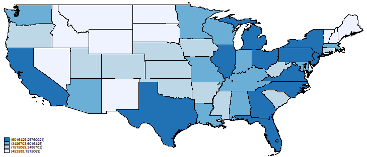
Right now, focus on what we typed:

	. spmap pop1990 using uscoord if id !=1 & id!=56, id(id) fcolor(Blues)

By default, a choropleth graph is drawn unless you specify the area() option. In a choropleth graph, different areas have different colors.

Let’s go over the command:

• using uscoord. Specifying using uscoord is not optional; spmap needs to know the name of the coordinates dataset. Remember, we used shp2dta to create two datasets—a database, which we merged with our statistical data, and a coordinate dataset, which we named uscoord.dta.
• id(id). Specifying id(id) is not optional. This is the name of the variable that identifies the locations. Earlier we told you to name the identification variable id. If you named it something else, you would specify the name that you used in the parentheses.
• fcolor(Blues). Specifying fcolor(Blues) really is optional. The Blues palette uses shades of blue for the colors.

In the command

	. spmap pop1990 using uscoord if id !=1 & id!=56, id(id) fcolor(Blues) 

we specified variable pop1990, and, in the dataset, that variable contains the population. The units do not matter; the data could just as well be coded in millions, and we would have obtained the same graph, although the legend would change.

By default, spmap divides the specified variable into four groups that are based on quartiles. You can change the number of groups by using option clnumber(#).

We will stick with four groups. In the spmap command, we used the if qualifier id !=1 & id!=56 to exclude Alaska and Hawaii from our graph because the map would have looked like this:

We also could exclude Alaska and Hawaii by typing

	. spmap pop1990 using uscoord if NAME!="Alaska" & NAME!="Hawaii", id(id) fcolor(Blues) 

because 56 and 1 are the id codes for Alaska and Hawaii and because our dataset happens to contain variable NAME, which records the name in string form.

Look closely at the legend, and you will see the population ranges are displayed in units of a thousand. We will change population to be recorded in millions with the following commands:

	. replace pop1990 = pop1990/1e+6

	. format pop1990 %4.2f

spmap has many options that control the color, legend, etc. Read about them in the online help file (type help spmap).

Friedrich Huebler’s blog, at http://huebler.blogspot.com, occasionally discusses spmap.