1 item has been added to your cart.

How can I create variables containing percent summaries?

Introduction

Many variables may be described as holding percentages. Such variables do not necessarily lie between 0 and 100, because percent changes may exceed 100 or fall below 0. This FAQ focuses on a special case, calculating mean percentages from indicator variables. On closer examination, the case is not as special as it looks, but it turns out to offer a key to unlocking more complicated problems.

Some comments on graphs of percent variables are also included in the last section.

Indicator variables and percentages

Suppose you have a table similar to the following for two categorical variables:

 . sysuse auto
 (1978 Automobile Data)
 . tabulate rep78 foreign, row

 +----------------+
 | Key            |
 |----------------|
 |   frequency    |
 | row percentage |
 +----------------+

      Repair |
      Record |       Car type
        1978 |  Domestic    Foreign |     Total
  -----------+----------------------+----------
   	   1 |         2          0 |         2
             |    100.00       0.00 |    100.00
  -----------+----------------------+----------
           2 |         8          0 |         8
             |    100.00       0.00 |    100.00
  -----------+----------------------+----------
           3 |        27          3 |        30
   	     |     90.00      10.00 |    100.00
  -----------+----------------------+----------
           4 |         9          9 |        18
   	     |     50.00      50.00 |    100.00
  -----------+----------------------+----------
           5 |         2          9 |        11
   	     |     18.18      81.82 |    100.00
  -----------+----------------------+----------
       Total |        48         21 |        69
   	     |     69.57      30.43 |    100.00

From the table we see, for example, that 81.82% of cars with repair record 5 are foreign and the other 18.18% are domestic. Expressed as proportions, these shares are 0.8182 and 0.1818. Focus first on foreign, which is an indicator variable (a.k.a., attribute, dichotomous, dummy, logical, quantal, Boolean, Bernoulli, or just plain binary) capable of taking on values of 0 or 1 (or missing). foreign is coded 0 for domestic cars and 1 for foreign cars.

Now suppose you want to get these percentages into variables for further analysis. First, know that egen, pc() does not do this; it just scales each value to be a percentage of its own total. The 11 observations with repair record 5 therefore have values 0, 0, 1, 1, 1, 1, 1, 1, 1, 1, 1 and total 9, so that

     . by rep78, sort: egen pc = pc(foreign)

produces two values of 0 and nine values of 100/9 or 11.11 to 2 d.p. for the 11 observations with repair record 5.

A useful idea here is that a mean percentage is just

100 * mean of a proportion

which in turn is just

100 * mean of an indicator variable

so that at its root the problem is one of calculating means. We need no special command or function to calculate percentages.

The 11 observations with repair record 5 have a mean of 9/11, or 0.8182 to 4 d.p., from which the percent foreign is 81.82 to 2 d.p., as already established. So, to get percent summaries from an indicator variable, simply

        . by rep78, sort: egen pc = mean(foreign)
	. replace pc = 100 * pc

and an even easier way is

        . by rep78, sort: egen pc = mean(100 * foreign)

Two principles are used here. The syntax diagram for egen, mean() states that it feeds on an expression, which can be more complex than just a variable name. An expression in this context is anything that evaluates to one number, which might be missing, for each observation. Thus 100 * foreign is just as acceptable here as foreign. Also

constant * mean of variable = mean of constant * variable

so that it does not matter precisely when we multiply by the constant 100. Doing it upstream here is easier than doing it downstream.

The same principles open the door for other, more complicated variants of this problem. What if we wanted percent domestic, not percent foreign? The crude solution is just calculating the complement

        . replace pc = 100 - pc

but a neater solution is doing it all in one:

        . by rep78, sort: egen pc = mean(100 * (1 - foreign))

We could tack on if or in conditions here and still use the same logic. However, what needs more care is the possibility of missing values.

To make things more challenging, suppose you want the percentage of good repair records, defined as 4 or 5, for the two categories of domestic and foreign cars. There are various ways we could calculate the corresponding indicator variable. Here are four:

 . generate good_record = rep78 == 4 | rep78 == 5
 . generate good_record = inlist(rep78, 4, 5)
 . generate good_record = inrange(rep78, 4, 5)
 . generate good_record = rep78 > 3

The principle here is that a true or false expression has a numeric value of 0 when false and 1 when true. See FAQ: "What is true and false in Stata?" for more details.

However we do it, keeping track of missing values can save you from some messes. In the auto dataset, repair record is missing in 5 observations. In the first three commands above, those missings would map to 0. In the last, they would map to 1 because missing is treated as larger than any known numeric value. To insist on a map from missing to missing, you need to spell out

        if rep78 < .

or

        if !mi(rep78)

The indicator variable, however, is not essential, and we can get the mean percentages directly with egen:

 . by foreign, sort: egen good_record =
 > mean(100 * inlist(rep78, 4, 5)) if rep78 < .
 . label var good_record "% with good record"
 . tabdisp foreign, cell(good_record) format(%3.1f)

 -------------------------------
   Car type | % with good record
 -----------+-------------------
   Domestic |               22.9
    Foreign |               85.7
 -------------------------------

A note on contract

The command contract can be useful for creating temporary datasets including a percent variable. Save your dataset beforehand. Alternatively, but with a higher risk, a preserve just before a keep or drop saves a copy of your current dataset, to which you can return on a restore given later in the same session. Typing

     . contract foreign rep78, zero freq(freq) percent(pc) 

illustrates the main possibilities. The resulting dataset includes new variables containing frequencies and percentages (the latter of the data as a whole) as well as cross combinations of the variables specified that have zero frequencies. The percent() option was added to contract to Stata 8 on 1 July 2004.

If you want other types of percentages and need to calculate them directly, the best way is through an application of by. For example,

     . by rep78 foreign, sort: generate freq = _N
     . by rep78: generate pc_rep78 = 100 * freq / _N 

produces the row percentages shown by tabulate rep78 foreign, row as given at the start of this document.

A note on graphs

Users often want to show a set of percent summaries, using, say, graph bar, graph hbar, or graph dot. At first sight, percentages of this kind are not among the reductions offered. But because percentages, apart from the factor of 100, are just means of indicator variables, having an indicator variable is enough to get a graph:

     . graph bar (mean) foreign, over(rep78)
     > ylabel(0 .2 "20" .4 "40" .6 "60" .8 "80") ytitle(Percent foreign cars)

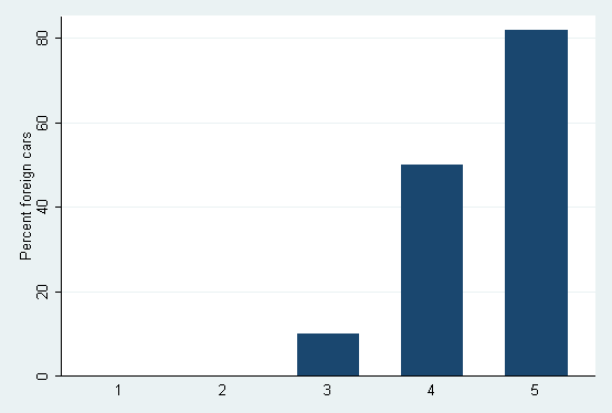
Here the percent issue is handled by axis labels and axis title. All graph bar knows is that it is graphing means.

If the percentages have been calculated already, it is often a good idea to try twoway bar.

     . twoway bar good_record foreign, xlabel(0 1, noticks valuelabel)
     > xscale(r(-0.5, 1.5)) barwidth(0.5) base(0)

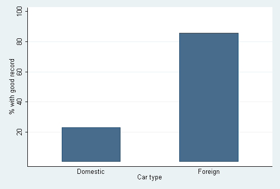
An advantage of twoway bar is it can be combined with other twoway graphs to produce customized displays. Thus if you want to graph percentages of one categorical variable as bars but also indicate the underlying total counts of the other categorical variable on top of each bar, you can do it as follows:

     . egen percent = mean(100 * foreign), by(rep78) 
     . egen total = total(1), by(rep78) 
     . twoway bar percent rep78, barw(0.5) || 
     > scatter percent rep78, mlabel(total) mlabpos(12) 
     > ms(none) legend(off) ytitle(percent foreign)

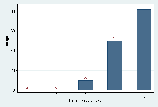
Here the scatter type shows invisible point symbols at the positions of the percents but also shows text from the variable total as marker labels. The option mlabpos(12) ensures a clock position of 12 o'clock, that is, just above the tops of the bars.

Finally, another possibility is the community-contributed catplot, which may be installed using ssc.

     . catplot foreign rep78, percent(rep78) asyvars stack
     > bar(1, bcolor(none)) bar(2, bcolor(green)) ytitle(percent breakdown)
     > ylabel(, angle(h)) recast(bar)

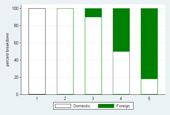
catplot's percent() option allows specification of one or more variables, so it is more flexible than contract in particular.