What’s new in multiple imputation

• New imputation features
• New estimation and postestimation features
• New data-management features

New imputation features

• The mi impute command now supports multivariate imputation using chained equations (ICE), mi impute chained, also known as sequential regression multivariate imputation (SRMI).
  
  ICE is a flexible imputation technique for imputing various types of data. The variable-by-variable specification of ICE allows you to impute variables of different types by choosing from several univariate imputation methods the appropriate one for each variable. Variables can have an arbitrary missing-data pattern. By specifying a separate model for each variable, you can incorporate certain important characteristics, such as ranges and restrictions within a subset, specific to each variable.
  
  
  
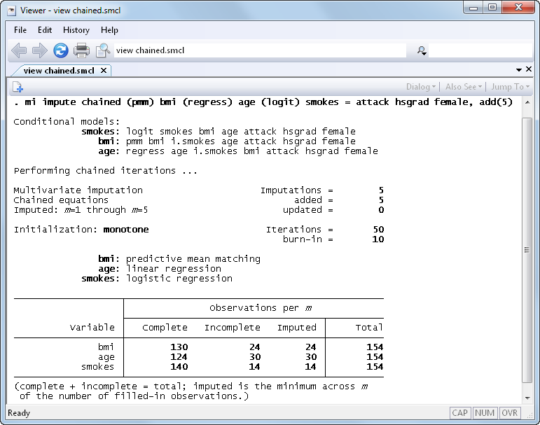
  Use any of nine univariate imputation methods to build a flexible imputation model.
  
  Customize prediction equations for imputed variables (for example, omit hsgrad from the model for bmi).
  
  Impute some variables using conditional imputation.
  
  Allow general expressions of imputed variables in the equations of other imputed variables (such as include bmi^2 in age’s imputation model).
• There are four new univariate imputation methods that can also be used as building blocks for multivariate imputation using the monotone method or the new chained-equations method.
  • mi impute truncreg imputes continuous variables with a restricted range using the truncated regression method
  • mi impute intreg imputes continuous censored variables using the interval regression method
  • mi impute poisson imputes count variables using the Poisson method
  • mi impute nbreg imputes overdispersed count variables using the negative binomial method
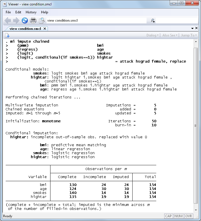
• Conditional imputation is now supported with all imputation techniques, except multivariate normal imputation (MVN), via the conditional() option.
  
  Conditional imputation allows you to impute variables which are defined within a particular subset of the data. Outside that subset, the variables are known to be constant. For example, the number of pregnancies is relevant only to females and is always zero for males, the smoking of high-tar cigarettes is relevant only to smokers and is always zero for nonsmokers.
  
  To properly impute, say, whether a person smokes high-tar cigarettes, we should condition on the smoking status during imputation. That is, we should impute missing values of subjects who smoke using only data on smokers and replace missing values of subjects who do not smoke with zeros. We would like to be able to do that even when the smoking status contains missing values and is itself being imputed. The conditional() option provides such capability:
  
  
  
• Separate imputation for different groups of the data is now available via mi impute's new by() option.
• Imputation by drawing posterior estimates from bootstrapped samples is now available with all imputation techniques, except MVN, via the new bootstrap option.
• Perfect prediction is now handled during imputation of categorical data using logistic, ordered logistic, or multinomial logistic imputation methods when the new augment option is specified.
• mi impute is now faster in the wide, mlong, and flong styles.

New estimation and postestimation features

• Estimate the amount of simulation error in your final model, so you can decide whether you need more imputations using mi estimate’s new mcerror option.
• mi estimate now supports panel-data and multilevel models. Included are xtcloglog, xtgee, xtlogit, xtmelogit, xtmepoisson, xtmixed, xtnbreg, xtpoisson, xtprobit, xtrc, and xtreg.
• mi estimate now supports the total command.
• Compute linear and nonlinear predictions after MI estimation using new commands mi predict and mi predictnl.

New data-management features

• misstable summarize will now create summary variables recording the missing-values pattern via the new generate() option.

Back to highlights

See New in Stata 12 for more about what was added in Stata Release 12.