1 item has been added to your cart.

Multiple imputation for missing data

Stata’s new mi command provides a full suite of multiple-imputation methods for the analysis of incomplete data, data for which some values are missing. mi provides both the imputation and the estimation steps. mi’s estimation step encompasses both estimation on individual datasets and pooling in one easy-to-use procedure. Features are provided to examine the pattern of missing values in the data. Flexible imputation methods are also provided, including five univariate imputation methods that can be used as building blocks for multivariate imputation, as well as multivariate normal (MVN).

mi provides easy importing of already imputed data and full imputed-data management capabilities.

Multiple imputation—estimation

We want to study the linear relationship between y and predictors x1 and x2. Our data contain missing values, however, and standard casewise deletion would result in a 40% reduction in sample size! We will fit the model using multiple imputation (MI).

First, we impute missing values and arbitrarily create five imputation datasets:

That done, we can fit the model:

mi estimate fits the specified model (linear regression here) on each of the imputation datasets (five here) and then combines the results into one MI inference.

Multiple imputation—nuts and bolts

mi can import already imputed data from NHANES or ice, or you can start with original data and form imputations yourself.

Either way, dealing with the multiple copies of the data is the bane of MI analysis. mi solves that problem. mi organizes the data in one of four formats, called wide, mlong, flong, and flongsep. In flongsep format, each imputation dataset is its own file. In the other formats, the data are combined into one dataset. Each format has its advantages, and mi makes it easy to switch formats. You can type or click one command to switch your data from one format to another. You can work with the data organized one way, continue with the data organized another, and so always work with the most convenient organization.

All mi commands work with all data formats.

Full data management is provided, too. You can create variables, drop variables, or create and drop observations as if you were working with one dataset, leaving it to mi to duplicate the changes correctly over each of the imputation datasets. You can merge your MI data with other datasets, both regular and MI, or append them, or copy the imputed values from one dataset to another. If you are analyzing survival data, you can split or join time periods just as you would ordinarily. The same applies if you are working with panel data and want to reshape your data. The fact that the actions you take might need to be carried out consistently over 5, 50, or even 500 datasets is irrelevant.

Multiple Imputation—Control Panel

mi’s Control Panel will guide you through all the phases of MI.

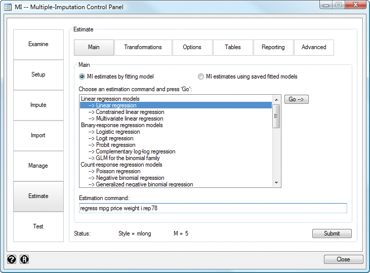
The Control Panel unifies many of mi’s capabilities into one flexible user interface. It guides you from the very beginning of your MI working session—examining missing values and their patterns—to the very end of it—performing MI inference.

Use the Examine tools to check missing-value patterns and to determine the appropriate imputation method.

Move on to Setup to set up your data for use by mi.

Need to create imputations? Use Impute.

Already have imputations? Skip Setup and go directly to Import to import your already imputed data.

To create new variables, merge or reshape your data, or use other data-management commands with mi data, go to Manage.

When you are ready, use Estimate to choose a model for your analysis. A set of dialog tabs will help you easily build your MI estimation model.

The Test panel lets you finish your analysis by performing tests of hypotheses.

Multiple imputation—capabilities

• Imputation
  
  
  1. Impute missing values of a single variable using one of five univariate methods:
     
     
     • linear regression (fully parametric) for continuous variables
     • predictive mean matching (partially parametric) for continuous variables
     • logistic for binary variables
     • ordered logit for ordinal variables
     • multinomial (polytomous) logistic for nominal variables
  2. Build a flexible model using any of the five methods above to impute missing values of multiple variables having a monotone missing-value pattern. (You could impute x1 and x2 jointly using predictive mean matching for x1 and ordered logistic for x2.)
     
     Customize prediction equations for imputed variables (such as omitting z2 from the model for x1).
     
     Impute missing values using different observations for different variables (such as imputing missing values of number of cigarettes smoked per day using only current smokers while using all observations to impute weight).
     
     Allow general expressions of imputed variables in the equations for later imputed variables (impute x1 and include x1² in x2’s imputation model).
  3. Impute missing values of multiple variables with an arbitrary missing-value pattern using an MVN model, allowing full or conditional model specification. Three prior specifications are provided.
  4. Update missing values even after you have already imputed some of them, including increasing the number of imputation datasets.
  5. Impute missing values using weighted and survey-weighted data with all the above techniques except MVN.
• Estimation
  
  
  1. In one simple step, perform both individual estimations and pooling of results.
  2. Fit models with most Stata estimation commands, including survival-data regression models and survey-data regression models.
  3. Obtain MI estimates of transformed parameters.
  4. Obtain MI estimates from previously saved individual estimation results.
  5. Obtain detailed information about MI characteristics, including relative efficiency and fraction of missing information due to nonresponse.
  6. Estimate with user-written estimators.
  7. mi verifies the integrity of the estimation model across imputations (consistency of estimation samples and omitted variables, model convergence) and notifies you if a problem exists.
• Postestimation
  
  
  1. Perform tests on multiple coefficients simultaneously.
  2. Tests available under the assumptions of equal and unequal fractions of missing information.
  3. Small-sample adjustments.

Explore more about multiple imputation in Stata.

Back to highlights