In the spotlight: Treatment effects
A delicate balancing act

Treatment-effects modeling is a fundamental tool to obtain experimental-style causal effects from observational data. Ideally, we would conduct an experiment, but for ethical or financial reasons, an experiment sometimes is not feasible.
A good example is the effect of cigarette smoking (the treatment) on the birthweight of infants (the outcome). In an experiment, we would first obtain a representative sample of pregnant women. Then, some would be told not to smoke (the control group), while others would be forced to smoke an arbitrary number of cigarettes per day (the treatment group). Clearly, such an experiment is unethical and would not be allowed. However, we can still answer our question of interest using Stata’s suite of parametric, semiparametric, and nonparametric treatment-effects estimators.
Suppose we want to tackle this question using teffects. For our estimates to be trustworthy, we have to guarantee that once we control for observable characteristics, it is as if pregnant mothers had been randomly assigned to control and treatment groups.
In an experiment, it is easy to inspect whether the characteristics of the treatment and control groups are equivalent. We simply need to look at the data as observed. For instance, the mothers in both groups should have the same age and level of education on average, and if we plotted the density of both groups, they should look the same.
However, this is not the case with observational data. Instead, we inspect whether our treatment-effects model reweights the data in such a way that the model-adjusted distribution of the mothers’ characteristics is equivalent across groups.
The balancing act in action
We model the birthweight (bweight) as a function of the number of prenatal visits (nprenatal), whether the mother is married (mmarried), and whether this baby is her first pregnancy (fbaby). The treatment, smoking during pregnancy (mbsmoke), is modeled as a function of the same variables and with regard to whether the mother consumed alcohol during her pregnancy. We type
. webuse cattaneo2, clear
(Excerpt from Cattaneo (2010) Journal of Econometrics 155: 138-154)

. teffects ipwra (bweight nprenatal i.mmarried i.fbaby)
                 (mbsmoke i.mmarried i.alcohol i.fbaby nprenatal)
We do not show the output, but suffice it to say that the effect of smoking is large and decidedly significant.
To obtain balancing diagnostics of the averages and variances of the mothers’ characteristics across groups, we type
. tebalance summarize
  Covariate balance summary
| Raw Weighted | |
| Number of obs = 4,642 4,642.0 | |
| Treated obs = 864 2,318.7 | |
| Control obs = 3,778 2,323.3 | |
| Standardized differences Variance ratio | ||
| Raw Weighted Raw Weighted | ||
| mmarried | ||
| married | -.5953009 -.0002835 1.335944 1.000247 | |
| alcohol | ||
| 1 | .3222725 -.0031106 4.509207 .9838918 | |
| fbaby | ||
| Yes | -.1663271 .0131381 .9430944 1.003143 | |
| nprenatal | -.2837987 -.0154989 1.430129 1.044148 | |
The values in the Raw columns show that without controlling for covariates, the groups are very different. The values in the Weighted columns show the differences in means and the ratio of the variances of the control and treatment groups after reweighting for the covariates. The mean differences are all near zero, and the variance ratios are all close to one. These diagnostics suggest that after we control for the covariates, it is as if we had randomly assigned the mothers to either the control group or the treatment group.
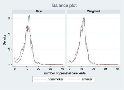
We can also inspect this graphically by plotting the distribution before fitting our model and the distribution after weighting. We do this for the number of prenatal visits.
. tebalance density nprenatal

The density graphs confirm what we observe from our diagnostics.
Can we do a test?
What we have described so far is qualitative: we have diagnostics but not a formal test. We can, however, do a test. Intuitively, the score equations for the treatment and control groups should be the same. We can test whether this is the case by using the score equations as moments in an overidentification test. The null hypothesis is that our covariates are balanced. We type
. tebalance overid
Overidentification test for covariate balance
         H0: Covariates are balanced:

         chi2(5)      =   4.0425
         Prob > chi2  =   0.5433
We cannot reject the null hypothesis. This implies that there is no evidence that our covariates remain imbalanced after reweighting.
Parting words
Sometimes, we cannot conduct experiments, but we can obtain experimental-style causal effects from observational data. For this to happen, we need to be able to say that our treatment-effects model reweights the data in such a way that the model-adjusted distribution of the covariates is equivalent across treatment groups. We can verify this with the postestimation diagnostic tests provided in teffects.
—Enrique Pinzon
Senior Econometrician, StataCorp


