Time series regression for counts allowing for autocorrelation in air pollution studies using Stata

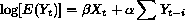
A main objective of the APHEA project (Katsouyanni, et al. 1995) was to develop and standardize a methodology for the detection of short-term effects of air pollution on health using epidemiological time series. Since the dependent variable, such as daily mortality, is a non-negative count, a Poisson regression was used. The model assumes

where is the matrix of predictor variables on day t with regression coefficients , is the number of deaths on day t, and E denotes the expected value. Time series data usually contains autocorrelation between the observations. The presence of autocorrelation is often an indication of incomplete or inadequate model specification since the reason for autocorrelation of the deaths is because they are conditional on autocorrelated predictor variables. If the model were correct, the residual autocorrelation should be minimal since one death does not cause another. Thus residual autocorrelation maybe implies confounding of air pollution associations due to unmeasured or mismodeled variables. The solution proposed in APHEA project was to include a specification of the autocorrelation in the model, and from this, standard Poisson regression needs to be modified. Following Schwartz et al. (1996) Poisson regression with autocorrelated residuals is suitable to analyze time studies controlling for autocorrelation. In this model the covariance matrix is defined as follows:

The code in arpois.ado fits this Poisson autoregressive model. Two types of autoregressive terms are allowed to be included in the model: studentized residuals

where , or lagged values of the dependent variable

The order of the autocorrelation could be empirically estimated examining the autocorrelation function plot. This option has been included in the code using the acplot.ado file developed by Cox (1997).

However, it should be recognized that these models could be may lead to instability of the estimated associations because the high day to day correlation of air pollution exposures. The inclusion of autocorrelation terms in the model is generally felt to produce a conservative estimate of the pollution effect size and standard error (Brunekreff et al. 1995).

References