Unobserved components model (UCM)

Stata’s ucm estimates the parameters of an unobserved components model (UCM). UCM decomposes a time series into trend, seasonal, cyclical, and idiosyncratic components and allows for exogenous variables. UCM is an alternative to ARIMA models and provides a flexible and formal approach to smoothing and decomposition problems.

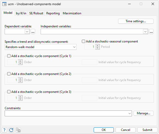
Here we fit monthly data on the median duration of unemployment spells in the United States to a stochastic cycle model with a stochastic seasonal component because the data have not been seasonally adjusted.

. webuse uduration2
(BLS data, not seasonally adjusted)

. ucm duration, seasonal(12) cycle(1) difficult

(output omitted)

Unobserved-components model
Components: random walk, seasonal(12), order 1 cycle

Sample: 1967m7 thru 2008m12                               Number of obs =    498
                                                          Wald chi2(2)  =   7.17
Log likelihood = -388.25675                               Prob > chi2   = 0.0277

 

     duration 
 
 Coefficient  Std. err.      z    P>|z|     [95% conf. interval]
 
 
 
    frequency 
 
   1.641531   .7250323     2.26   0.024     .2204938    3.062568
      damping 
 
   .2671232   .1050168     2.54   0.011     .0612939    .4729524
 
 
 
    var(level)
 
   .1262922   .0221428     5.70   0.000     .0828932    .1696912
 var(seasonal)
 
   .0017289   .0009647     1.79   0.037            0    .0036196
   var(cycle1)
 
   .0641496   .0211839     3.03   0.001     .0226299    .1056693

Note: Model is not stationary.
Note: Tests of variances against zero are one sided, and the two-sided
      confidence intervals are truncated at zero.

Important components are components with a large spectral density, and, thus, the estimated damping parameter specifies how tightly the important components are distributed around the estimated central frequency. We calculate and plot the spectral density implied by these parameter estimates below.

. psdensity omega density

. twoway line omega density

Moving on to prediction, we predict the trend and the seasonal components:

. predict strend, trend

. predict season, seasonal

Below we graph the trend component in the top panel and the seasonal component in the bottom panel.

We can also forecast the median unemployment duration and graph the results.

. tsappend, add(12)

. predict duration_f, dynamic(tm(2009m1)) rmse(rmse)