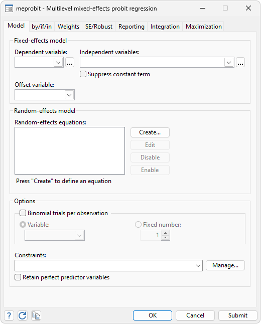
Stata allows you to fit multilevel mixed-effects probit models with meprobit. A multilevel mixed-effects probit model is an example of a multilevel mixed-effects generalized linear model (GLM). You can fit the latter in Stata using meglm.

Let's fit a crossed-effects probit model. A crossed-effects model is a multilevel model in which the levels of random effects are not nested. We investigate the extent to which two salamander populations, whiteside and roughbutt, cross-breed. We label whiteside males wsm, whiteside females wsf, roughbutt males rbm, and roughbutt females rbf. Our dependent variable y is coded 1 if there was a successful mating and 0 otherwise. Let's fit our model:
. webuse salamander

. meprobit y wsm##wsf || _all: R.male || female:
note: crossed random-effects model specified; option intmethod(laplace) implied.

Fitting fixed-effects model:

Iteration 0:  Log likelihood = -223.01026
Iteration 1:  Log likelihood = -222.78736
Iteration 2:  Log likelihood = -222.78735

Refining starting values:

Grid node 0:  Log likelihood = -216.49485

Fitting full model:

Iteration 0:  Log likelihood = -216.49485  (not concave)
Iteration 1:  Log likelihood = -214.34477  (not concave)
Iteration 2:  Log likelihood = -212.35196
Iteration 3:  Log likelihood =  -209.7382
Iteration 4:  Log likelihood = -208.37212
Iteration 5:  Log likelihood = -208.34892
Iteration 6:  Log likelihood =  -208.2553
Iteration 7:  Log likelihood = -208.11499
Iteration 8:  Log likelihood = -208.11233
Iteration 9:  Log likelihood = -208.11182
Iteration 10: Log likelihood = -208.11182

Mixed-effects probit regression                 Number of obs     =        360

        Grouping information


      No. of       Observations per group
 Group variable       groups    Minimum    Average    Maximum

           _all            1        360      360.0        360
         female           60          6        6.0          6


Integration method: laplace

                                                Wald chi2(3)      =      40.46
Log likelihood = -208.11182                     Prob > chi2       =     0.0000
| y | Coefficient Std. err. z P>|z| [95% conf. interval] | |
| 1.wsm | -.4122043 .2734728 -1.51 0.132 -.9482011 .1237925 | |
| 1.wsf | -1.720331 .327954 -5.25 0.000 -2.36311 -1.077553 | |
| wsm#wsf | ||
| 1 1 | 2.121125 .3647297 5.82 0.000 1.406268 2.835982 | |
| _cons | .5950965 .2360978 2.52 0.012 .1323533 1.05784 | |
| _all>male | ||
| var(_cons) | .3867458 .1795526 .1556835 .9607463 | |
| female | ||
| var(_cons) | .446411 .199398 .1860071 1.071372 | |
Our model has two random-effects equations, separated by ||. We use the _all notation that identifies all the observations as one big group. We use the R. notation to tell Stata to treat male as an indicator variable.
The output table includes the fixed-effect portion of our model and the estimated variance components. The estimates of the random intercepts suggest that the heterogeneity among the female salamanders is larger than the heterogeneity among the male salamanders.
If we wish, we can constrain the two random intercepts to be equal.
. constraint 1 _b[/var(_cons[_all>male])] = _b[/var(_cons[female])]

. meprobit y wsm##wsf || _all: R.male || female:, constraint(1) nolog
note: crossed random-effects model specified; option intmethod(laplace)
      implied.

Mixed-effects probit regression                 Number of obs     =        360

        Grouping information


      No. of       Observations per group
 Group variable      groups    Minimum    Average    Maximum

           _all           1        360      360.0        360
         female          60          6        6.0          6


Integration method: laplace

                                                Wald chi2(3)      =      40.12
Log likelihood = -208.14476                     Prob > chi2       =     0.0000
 ( 1)  [/]var(_cons[_all>male]) - [/]var(_cons[female]) = 0
| y | Coefficient Std. err. z P>|z| [95% conf. interval] | |
| 1.wsm | -.4130233 .2945617 -1.40 0.161 -.9903537 .1643071 | |
| 1.wsf | -1.720578 .3294304 -5.22 0.000 -2.36625 -1.074907 | |
| wsm#wsf | ||
| 1 1 | -1.720578 .3294304 -5.22 0.000 -2.36625 -1.074907 | |
| _cons | .5963019 .2514219 2.37 0.018 .103524 1.08908 | |
| _all>male | ||
| var(_cons) | .4156124 .1500219 .204849 .8432244 | |
| female | ||
| var(_cons) | .4156124 .1500219 .204849 .8432244 | |
You can also fit our model using a logit model (see melogit) or a complementary log-log model (see mecloglog).
Also watch A tour of multilevel GLMs.