|
|

Under the heading least squares, Stata can fit ordinary regression models, instrumental-variables models, constrained linear regression, nonlinear least squares, and two-stage least-squares models. (Stata can also fit quantile regression models, which include median regression or minimization of the absolute sums of the residuals.)
After fitting a linear regression model, Stata can calculate predictions, residuals, standardized residuals, and studentized (jackknifed) residuals; the standard error of the forecast, prediction, and residuals; the influence measures Cook’s distance, COVRATIO, DFBETAs, DFITS, leverage, and Welsch’s distance; variance-inflation factors; specification tests; and tests for heteroskedasticity.
Among the fit diagnostic tools are added-variable plots (also known as partial-regression leverage plots, partial regression plots, or adjusted partial residual plots), component-plus-residual plots (also known as augmented partial residual plots), leverage-versus-squared-residual plots (or L-R plots), residual-versus-fitted plots, and residual-versus-predictor plots (or independent variable plots). Each tool is available by typing one command.
For example, let’s start with a dataset that contains the price, weight, mpg, and origin (foreign or U.S.) for 74 cars:
. webuse auto
(1978 automobile data)

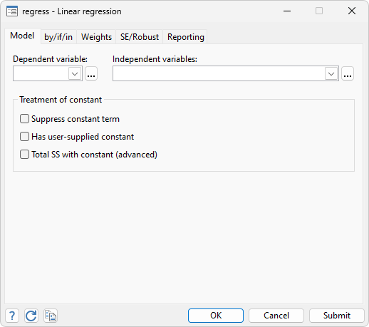
. regress price weight foreign##c.mpg
| Source | SS df MS | Number of obs = 74 | |
| F(4, 69) = 21.22 | |||
| Model | 350319665 4 87579916.3 | Prob > F = 0.0000 | |
| Residual | 284745731 69 4126749.72 | R-squared = 0.5516 | |
| Adj R-squared = 0.5256 | |||
| Total | 635065396 73 8699525.97 | Root MSE = 2031.4 |
| price | Coefficient Std. err. t P>|t| [95% conf. interval] | |
| weight | 4.613589 .7254961 6.36 0.000 3.166263 6.060914 | |
| foreign | ||
| Foreign | 11240.33 2751.681 4.08 0.000 5750.878 16729.78 | |
| mpg | 263.1875 110.7961 2.38 0.020 42.15527 484.2197 | |
| foreign#c.mpg | ||
| Foreign | -307.2166 108.5307 -2.83 0.006 -523.7294 -90.70368 | |
| _cons | -14449.58 4425.72 -3.26 0.002 -23278.65 -5620.51 | |
We have used factor variables
in the above example. The term foreign##c.mpg specifies to include
a full factorial of the variables—main effects for each variable and an
interaction. The c. just says that mpg is continuous.
regress is Stata’s linear
regression command. All estimation commands have the same syntax: the name
of the dependent variable followed by the names of the independent variables.
After estimation, we can review diagnostic plots:
. rvfplot, yline(0)
Typing rvfplot displays a residual-versus-fitted plot, although we created the graph above by typing rvfplot, yline(0); this drew a line across the graph at 0. That you can discern a pattern indicates that our model has problems.
We obtain a leverage plot by typing:
. lvr2plot
avplot draws added-variable plots, both for variables currently in the model and variables not yet in the model:
. avplot mpg
Added-variable plots are so useful that they are worth reviewing for every variable in the model:
. avplots
The graph above is one Stata image and was created by typing avplots. The combined graph is useful because we have only four variables in our model, although Stata would draw the graph even if we had 798 variables in our model. The individual graphs would, however, be too small to be useful. That is why there is an avplot command.
Exploring the influence of observations in other ways is equally easy. For instance, we could obtain a new variable called cook containing Cook’s distance and then list suspicious observations by typing
. predict cook, cooksd, if e(sample)

. predict e if e(sample), resid

. list make price e cook if cook>4/74
| make price e cook | |||
| 12. | Cad. Eldorado 14,500 7271.96 .1492676 | ||
| 13. | Cad. Seville 15,906 5036.348 .3328515 | ||
| 24. | Ford Fiesta 4,389 3164.872 .0638815 | ||
| 28. | Linc. Versailles 13,466 6560.912 .1308004 | ||
| 42. | Plym. Arrow 4,647 -3312.968 .1700736 | ||
We could obtain all the DFBETAs and then list the four observations having the most negative influence on the foreign coefficient and the four observations having the most positive influence by typing
. dfbeta
Generating DFBETA variables ...

    _dfbeta_1: DFBETA weight
    _dfbeta_2: DFBETA 1.foreign
    _dfbeta_3: DFBETA mpg
    _dfbeta_4: DFBETA 1.foreign#c.mpg

. sort _dfbeta_2

. list make price foreign _dfbeta_2 in 1/4
| make price foreign _dfbeta_2 | |||
| 1. | Plym. Arrow 4,647 Domestic -.6622424 | ||
| 2. | Cad. Eldorado 14,500 Domestic -.5290519 | ||
| 3. | Linc. Versailles 13,466 Domestic -.5283729 | ||
| 4. | Toyota Corona 5,719 Foreign -.256431 | ||
| make price foreign _dfbet~2 | |||
| 71. | Volvo 260 11,995 Foreign .2318289 | ||
| 72. | Plym. Champ 4,425 Domestic .2371104 | ||
| 73. | Peugeot 604 12,990 Foreign .2552032 | ||
| 74. | Cad. Seville 15,906 Domestic .8243419 | ||