Dynamic-factor models

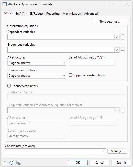
Stata’s dfactor estimates the parameters of dynamic-factor models by maximum likelihood. Dynamic-factor models are flexible models for multivariate time series in which the observed endogenous variables are linear functions of exogenous covariates and unobserved factors, which have a vector autoregressive structure. The unobserved factors may also be a function of exogenous covariates. The disturbances in the equations for the dependent variables may be autocorrelated.

We have data on industrial production (ipman), real disposable income (income), weekly hours worked (hours), and the unemployment rate (unemp). We suspect there exists a latent factor that can explain all four of these series, and we conjecture that latent factor follows an AR(2) process.

The first step is to fit our model:

. webuse dfex
(St. Louis Fed (FRED) macro data)

. dfactor (D.(ipman income hours unemp) =, noconstant) (f=, ar(1/2)), nolog

Dynamic-factor model

Sample: 1972m2 thru 2008m11                              Number of obs =    442
                                                         Wald chi2(6)  = 751.95
Log likelihood = -662.09507                              Prob > chi2   = 0.0000



               
 
 Coefficient  Std. err.      z    P>|z|     [95% conf. interval]
 
 
 
f              
 
             f 
 
           L1. 
 
   .2651932   .0568663     4.66   0.000     .1537372    .3766491
           L2. 
 
   .4820398   .0624635     7.72   0.000     .3596136     .604466
 
 
 
D.ipman        
 
             f 
 
   .3502249   .0287389    12.19   0.000     .2938976    .4065522
 
 
 
D.income       
 
             f 
 
   .0746338   .0217319     3.43   0.001     .0320401    .1172276
 
 
 
D.hours        
 
             f 
 
   .2177469   .0186769    11.66   0.000     .1811407     .254353
 
 
 
D.unemp        
 
             f 
 
  -.0676016   .0071022    -9.52   0.000    -.0815217   -.0536816
 
 
 
/observable    
 
  var(De.ipman)
 
   .1383158   .0167086     8.28   0.000     .1055675    .1710641
 var(De.income)
 
   .2773808   .0188302    14.73   0.000     .2404743    .3142873
  var(De.hours)
 
   .0911446   .0080847    11.27   0.000     .0752988    .1069903
  var(De.unemp)
 
   .0237232   .0017932    13.23   0.000     .0202086    .0272378

Note: Tests of variances against zero are one sided, and the two-sided
      confidence intervals are truncated at zero.

With our model fit, let’s obtain dynamic forecasts for disposable income beginning in December 2008:

. tsappend, add(3)

. predict income_f, dynamic(tm(2008m12))

. tsline D.income income_f if month >= tm(2005m1)

Even more interesting is the path of our unobserved factor. We have hypothesized that all our observed variables follow the unobserved latent factor. We can obtain the one-step predictions of the factor by typing

. predict factor, factor

We can then trace the path of the factor by graphing the result:

. tsline factor

Extracting the latent factor in this manner is sometimes referred to as extracting or estimating an indicator.

dfactor also estimates the parameters of static-factor models, seemingly unrelated regression (SUR) models, and vector autoregressive (VAR) models by maximum likelihood. dfactor allows for constraints on the covariance matrix of the errors in an SUR model and a VAR model.

After estimation, you can predict both the endogenous variables and the unobserved factors. In addition to one-step predictions, dfactor can produce dynamic multistep predictions.

Explore more time-series features in Stata.