The use of panel-data models has exploded in the past ten years as analysts more often need to analyze richer data structures. Some examples of panel data are nested datasets that contain observations of smaller units nested within larger units. An example might be counties (the replication) in various states (the panel identifier). Other examples of panel data are longitudinal, having multiple observations (the replication) on the same experimental unit (the panel identifier) over time. xtgee allows either type of panel data.
Stata estimates extensions to generalized linear models in which you can model the structure of the within-panel correlation. This extension allows users to fit GLM-type models to panel data.
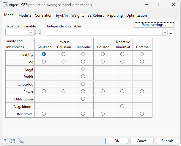
xtgee offers a rich collection of models for analysts. These models correspond to population-averaged (or marginal) models in the panel-data literature.
What makes xtgee useful is the number of statistical models that it generalizes for use with panel data, the richer correlation structure with models available in other commands, and the availability of robust standard errors, which do not always exist in the equivalent command.
In this example, we consider a probit model in which we wish to model whether a worker belongs to the union based on the person's age and whether they are living outside of an SMSA. The people in the study appear multiple times in the dataset (this type of panel dataset is commonly referred to as a longitudinal dataset), and we assume that the observations on a given person are more correlated than those between different persons.
. webuse nlswork
(National Longitudinal Survey of Young Women, 14-24 years old in 1968)

. xtset idcode

Panel variable: idcode (unbalanced)

. xtgee union age not_smsa, family(binomial) link(probit) corr(exchangeable)

Iteration 1: tolerance = .05859927
Iteration 2: tolerance = .00346479
Iteration 3: tolerance = .0001277
Iteration 4: tolerance = 4.486e-06
Iteration 5: tolerance = 1.548e-07

GEE population-averaged model                        Number of obs    = 19,226
Group variable: idcode                               Number of groups =  4,150
Family: Binomial                                     Obs per group:
Link:   Probit                                                    min =      1
Correlation: exchangeable                                         avg =    4.6
                                                                  max =     12
                                                     Wald chi2(2)     =  30.23
Scale parameter = 1                                  Prob > chi2      = 0.0000
| union | Coefficient Std. err. z P>|z| [95% conf. interval] | ||||||
| age | .0045624 .0013959 3.27 0.001 .0018264 .0072984 | ||||||
| not_smsa | -.1440246 .0318838 -4.52 0.000 -.2065156 -.0815336 | ||||||
| _cons | -.8770284 .0479603 -18.29 0.000 -.9710288 -.7830279 | ||||||
xtgee allows these options:
Families
|
Links
|
Correlation structures
|
Assume an independent correlation structure that ignores the panel structure of the data. Under this assumption, xtgee will produce answers already provided by Stata’s nonpanel estimation commands. Examples of situations when xtgee provides the same answers are given in the table shown below.
| Family | Link | Correlation | Equivalent Stata |
| gaussian | identity | independent | regress |
| gaussian | identity | exchangeable | xtreg, re |
| gaussian | identity | exchangeable | xtreg, pa |
| binomial | cloglog | independent | cloglog (see note 1) |
| binomial | cloglog | exchangeable | xtcloglog, pa |
| binomial | logit | independent | logit or logistic |
| binomial | logit | exchangeable | xtlogit, pa |
| binomial | probit | independent | probit (see note 2) |
| binomial | probit | exchangeable | xtprobit, pa |
| nbinomial | nbinomial | independent | nbreg (see note 3) |
| poisson | log | independent | poisson |
| poisson | log | exchangeable | xtpoisson, pa |
| gamma | log | independent | streg, dist(exp) nohr (see note 4) |
| family | link | independent | glm, irls (see note 5) |
| Note 1 | For cloglog estimation, xtgee with corr(independent) and cloglog will produce the same coefficients, but the standard errors will be only asymptotically equivalent because cloglog is not the canonical link for the binomial family. |
| Note 2 |
For probit estimation, xtgee with corr(independent) and probit will produce the same coefficients, but the standard errors will be only asymptotically equivalent because probit is not the canonical link for the binomial family. If the binomial denominator is not 1, the equivalent maximum-likelihood command is bprobit. |
| Note 3 | Fitting a negative binomial model using xtgee (or glm) will yield results conditional on the specified value of alpha. nbreg, however, estimates that parameter and provides unconditional estimates. |
| Note 4 |
xtgee with corr(independent) can be used to fit exponential regressions, but this requires specifying scale(1). As with probit, the xtgee-reported standard errors will be only asymptotically equivalent to those produced by streg, dist(exp) nohr because log is not the canonical link for the gamma family. xtgee cannot be used to fit exponential regressions on censored data. Using the independent correlation structure, xtgee will fit the same model as the glm, irls command if the family–link combination is the same. |
| Note 5 |
If xtgee is equivalent to another command, using corr(independent) and the vce(robust) option with xtgee corresponds to using vce(cluster clustvar) option in the equivalent command, where clustvar corresponds to the panel variable. |
If you choose to model the intracluster correlation as an identity matrix
(by specifying the name of an existing identity matrix in the option
corr), GEE estimation reduces to a generalized linear model, and the
results will be identical to estimation by glm.
. glm union age not_smsa, family(gauss) link(identity)

Iteration 0:  Log likelihood = -10713.086

Generalized linear models                         Number of obs   =     19,226
Optimization     : ML                             Residual df     =     19,223
                                                  Scale parameter =   .1784791
Deviance         =  3430.904127                   (1/df) Deviance =   .1784791
Pearson          =  3430.904127                   (1/df) Pearson  =   .1784791

Variance function: V(u) = 1                       [Gaussian]
Link function    : g(u) = u                       [Identity]

                                                  AIC             =   1.114749
Log likelihood   = -10713.08631                   BIC             =  -186185.1
| OIM | |||||||
| union | Coefficient std. err. z P>|z| [95% conf. interval] | ||||||
| age | .0018369 .0004926 3.73 0.000 .0008714 .0028024 | ||||||
| not_smsa | -.0648492 .0067672 -9.58 0.000 -.0781126 -.0515858 | ||||||
| _cons | .1950571 .0158061 12.34 0.000 .1640777 .2260365 | ||||||
| union | Coefficient Std. err. z P>|z| [95% conf. interval] | ||||||
| age | .0018369 .0004926 3.73 0.000 .0008715 .0028023 | ||||||
| not_smsa | -.0648492 .0067666 -9.58 0.000 -.0781116 -.0515869 | ||||||
| _cons | .1950571 .0158049 12.34 0.000 .1640801 .2260341 | ||||||
We could fill up lots of space demonstrating other ways that xtgee is equivalent to other features of Stata, but the real power is in using it for its intended use and modeling the correlation that exists in the panels.


