Balanced and unbalanced designs
Missing cells
Factorial, nested, and mixed designs
Repeated measures
Box, Greenhouse–Geisser, and Huynh–Feldt corrections
Afifi and Azen (1979) fitted a model of the change in systolic blood pressure for 58 patients, each suffering from one of three diseases, who were randomly assigned one of four different drug treatments:
. webuse systolic
(Systolic Blood Pressure Data)
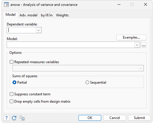
. anova systolic drug disease drug#disease
Number of obs = 58 R-squared = 0.4560
Root MSE = 10.5096 Adj R-squared = 0.3259
| Source | Partial SS df MS F Prob > F | ||||||
| Model | 4259.3385 11 387.21259 3.51 0.0013 | ||||||
| drug | 2997.4719 3 999.15729 9.05 0.0001 | ||||||
| disease | 415.87305 2 207.93652 1.88 0.1637 | ||||||
| drug#disease | 707.26626 6 117.87771 1.07 0.3958 | ||||||
| Residual | 5080.8167 46 110.45254 | ||||||
| Total | 9340.1552 57 163.86237 | ||||||
An important feature of Stata is that it does not have modes or modules. You do not enter the ANOVA module to fit an ANOVA model. The advantage in this is that all Stata’s features can be interspersed to help you better understand these data. For instance, the data here are almost balanced, as revealed by Stata's table:
. table drug disease
| Patient's Disease | ||||||
| 1 2 3 Total | ||||||
| Drug used | ||||||
| 1 | 6 4 5 15 | |||||
| 2 | 5 4 6 15 | |||||
| 3 | 3 5 4 12 | |||||
| 4 | 5 6 5 16 | |||||
| Total | 19 19 20 58 | |||||
table can also be used to help you better understand the relationship of the increase in blood pressure by drug and disease:
.table drug disease, statistic(mean systolic) nformat(%8.2f) style(table-right)
| Patient's Disease | ||||||
| 1 2 3 Total | ||||||
| Drug used | ||||||
| 1 | 29.33 28.25 20.40 26.07 | |||||
| 2 | 28.00 33.50 18.17 25.53 | |||||
| 3 | 16.33 4.40 8.50 8.75 | |||||
| 4 | 13.60 12.83 14.20 13.50 | |||||
| Total | 22.79 18.21 15.80 18.88 | |||||
Stata's test allows you to perform tests directly on the coefficients of the underlying regression model. For instance, we can test if the coefficient on the third drug is equal to the coefficient on the fourth.
. test 3.drug = 4.drug

 ( 1)  3.drug - 4.drug = 0

       F(  1,    46) =    0.13
            Prob > F =    0.7234
We find that the two coefficients are not significantly different, at least at any significance level smaller than 73%.
For more complex tests, contrast often provides a more concise way to specify the test we are interested in and prevents us from having to write tests in terms of the regression coefficients. With contrast, we instead specify our tests in terms of differences in the marginal means for the levels of a particular factor. For example, if we want to compare the third and fourth drugs, we can test the difference in the mean impact on systolic blood pressure separately for each disease using the @ operator. We also use the reverse adjacent operator, ar., to compare the fourth level of the drug with the previous level.
. contrast ar4.drug@disease

Contrasts of marginal linear predictions

Margins      : asbalanced
| df F P>F | ||||
| drug@disease | ||||
| (4 vs 3) 1 | 1 0.13 0.7234 | |||
| (4 vs 3) 2 | 1 1.76 0.1917 | |||
| (4 vs 3) 3 | 1 0.65 0.4230 | |||
| Joint | 3 0.85 0.4761 | |||
| Denominator | 46 | |||
| Contrast Std. Err. [95% Conf. Interval] | |||||
| drug@disease | |||||
| (4 vs 3) 1 | -2.733333 7.675156 -18.18262 12.71595 | ||||
| (4 vs 3) 2 | 8.433333 6.363903 -4.376539 21.24321 | ||||
| (4 vs 3) 3 | 5.7 7.050081 -8.491077 19.89108 | ||||
test and contrast can still access the estimates, even though two tabulations have intervened. Similarly, anova is integrated with Stata’s regress for estimating linear regressions. We can review the underlying regression estimates by typing regress without arguments:
. regress
| Source | SS df MS | Number of obs = 58 | |
| F( 11, 46) = 3.51 | |||
| Model | 4259.33851 11 387.212591 | Prob > F = 0.0013 | |
| Residual | 5080.81667 46 110.452536 | R-squared = 0.4560 | |
| Adj R-squared = 0.3259 | |||
| Total | 9340.15517 57 163.862371 | Root MSE = 10.51 |
| systolic | Coef. Std. Err. t P>t| [95% Conf. Interval] | |||||
| drug | ||||||
| 2 | -1.333333 6.363903 -0.21 0.835 -14.14321 11.47654 | |||||
| 3 | -13 7.431438 -1.75 0.087 -27.95871 1.958708 | |||||
| 4 | -15.73333 6.363903 -2.47 0.017 -28.54321 -2.923461 | |||||
| disease | ||||||
| 2 | -1.083333 6.783944 -0.16 0.874 -14.7387 12.57204 | |||||
| 3 | -8.933333 6.363903 -1.40 0.167 -21.74321 3.876539 | |||||
| drug#disease | ||||||
| 2 2 | 6.583333 9.783943 0.67 0.504 -13.11072 26.27739 | |||||
| 2 3 | -.9 8.999918 -0.10 0.921 -19.0159 17.2159 | |||||
| 3 2 | -10.85 10.24353 -1.06 0.295 -31.46916 9.769157 | |||||
| 3 3 | 1.1 10.24353 0.11 0.915 -19.51916 21.71916 | |||||
| 4 2 | .3166667 9.301675 0.03 0.973 -18.40663 19.03997 | |||||
| 4 3 | 9.533333 9.202189 1.04 0.306 -8.989712 28.05638 | |||||
| _cons | 29.33333 4.290543 6.84 0.000 20.69692 37.96975 | |||||
In our original estimation, the direct effect of disease was found to be insignificant, as was the drug#disease interaction. We might now compare our two-way factorial model with a simpler, one-way layout:
. test disease drug#disease
| Source | Partial SS df MS F Prob > F | |
| disease drug#disease | 1126.1 8 140.7625 1.27 0.2801 | |
| Residual | 5080.8167 46 110.45254 |
With the test example above, we found that a one-way model fits these data well. We could use either Stata's anova or Stata’s oneway to fit a one-way model.
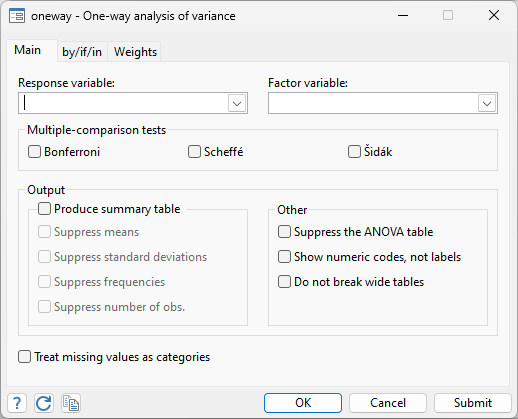
. oneway systolic drug, bonferroni
| Analysis of Variance | |||||
| Source SS df MS F Prob > F | |||||
| Between groups 3133.23851 3 1044.41284 9.09 0.0001 | |||||
| Within groups 6206.91667 54 114.942901 | |||||
| Total 9340.15517 57 163.862371 | |||||
| Bartlett's test for equal variances: chi2(3) = 1.0063 Prob>chi2 = 0.800 |
| Comparison of Increment in Systolic B.P. by Drug Used |
| (Bonferroni) |
| Row Mean- | ||||
| Col Mean | 1 2 3 | |||
| 2 | -.533333 | |||
| 1.000 | ||||
| 3 | -17.3167 -16.7833 | |||
| 0.001 0.001 | ||||
| 4 | -12.5667 -12.0333 4.75 | |||
| 0.012 0.017 1.000 | ||||
Table 7.7 of Winer, Brown, and Michels (1991) provides a repeated-measures ANOVA example involving both nested and crossed terms. There are four dial shapes and two methods for calibrating dials. Subjects are nested within the calibration method, and an accuracy score is obtained.
Here is Stata's anova for this problem.
. webuse t77
(T7.7 -- Winer, Brown, Michels)

. anova score calib / subject|calib shape calib#shape , repeated(shape)

                           	 Number of obs =      24     R-squared     =  0.8925
                           	 Root MSE      = 1.11181     Adj R-squared =  0.7939
| Source | Partial SS df MS F Prob > F | ||||||
| Model | 123.125 11 11.1931818 9.06 0.0003 | ||||||
| calib | 51.0416667 1 51.0416667 11.89 0.0261 | ||||||
| subject|calib | 17.1666667 4 4.29166667 | ||||||
| shape | 47.4583333 3 15.8194444 12.80 0.0005 | ||||||
| calib#shape | 7.45833333 3 2.48611111 2.01 0.1662 | ||||||
| Residual | 14.8333333 12 1.23611111 | ||||||
| Total | 137.958333 23 5.99818841 | ||||||
| ------------ | Prob > F | ------------ | |||||
| Source | df F Regular H-F G-G Box | ||||||
| shape | 3 12.80 0.0005 0.0011 0.0099 0.0232 | ||||||
| calib#shape | 3 2.01 0.1662 0.1791 0.2152 0.2291 | ||||||
| Residual | 12 | ||||||
Afifi, A. A., and S. P. Azen. 1979. Statistical Analysis: A computer-oriented approach. 2nd ed. New York: Academic Press.
Winer, B. J., R. Brown, and K. M. Michels. 1991. Statistical Principles in Experimental Design. 3rd ed. New York: McGraw–Hill.


