Meta-analysisNew using Stata
Houssein Assaad
Senior Statistician and Software Developer
StataCorp LLC
Webinar
April 28, 2020

Outline
- What is meta-analysis? Why and when you should use it ?
- Data setup: Effect-sizes and Meta-analysis models
- The meta suite: Exploring the syntax
- Examples: Two case studies
- Summary
- Meta-regression and subgroup-analysis:
- Publication bias: NSAIDS data
- The meta control panel
- BCG vaccine efficacy against tuberculosis
- MA is the science of combining results from multiple studies addressing a similar scientific question
What is meta-analysis (MA) ?
- MA has been mostly used in medicine, but also in econometrics, ecology, psychology, and education to name a few
- The goal of MA is to explore consistencies and discrepancies among the studies , and if sensible, provide a unified conclusion
- Potential problem: Publication bias, which occur when the results of the published literature in a certain domain differ systematically in its results from all the relevant research results
Why would you want to use meta-analysis ?
- An increase in power and improvement in precision
- The ability to answer questions not posed by individual studies
- The opportunity to settle controversies arising from conflicting claims
Potential advantages of MA include:
Data setup
- \(K\) studies
treatment group
control group
- Study \(j\) estimates effect size, \(\theta_j\) and its standard error \(\sigma_j\)
- Effect size (ES): a value that reflects the magnitude of group differences or the strength of a relationship between 2 variables
vs
ES
e.g. OR, RR, RD, Hedges's \(g\), Cohen's \(d\) etc.

variable 1
variable 2
ES
e.g. correlation coef. \(r\), regression coef \(\beta\) etc.
MA models
\(K\) independent studies, each reports:
- An estimate, \(\hat{\theta}_j\), of the true (unknown) effect size \(\theta_j\)
- An estimate, \(\hat{\sigma}_j\) , of its standard error
| Model | Assumption | Target of inference |
|---|---|---|
| common effect (CE) | common value |
|
| fixed effects (FE) | fixed | |
| Random effects (RE) |
- Estimating \(\theta\) (and \(\tau^2\) with RE model) is one of the main goals of MA
MA models
- All models use a weighted average of the study-specific effect sizes, but differ in how they define the weights \(w_j\)
- FE and CE models use \(w_j = 1/\hat{\sigma}_j^2\)
- RE models use \(w_j = 1/\left(\hat{\sigma}_j^2\ + \hat{\tau}^2\right)\), 7 estimation methods are supported to estimate \(\tau^2\)
     +--------------+
     |  es    se    |
     |--------------|
  1. | 2.4    .6    |
  2. | 1.3    .6    |
  3. | -.7    .5    |
  4. | 1.8   1.1    |
     |--------------|
  5. | 2.2   1.7    |
  6. | 1.2    .1    |
  7. |  .7    .2    |
     +--------------+
     +---------------------------------+
     |  es    se         w        w*es |
     |---------------------------------|
  1. | 2.4    .6     2.778       6.667 |
  2. | 1.3    .6     2.778       3.611 |
  3. | -.7    .5         4        -2.8 |
  4. | 1.8   1.1      .826       1.487 |
     |---------------------------------|
  5. | 2.2   1.7      .346        .761 |
  6. | 1.2    .1       100         120 |
  7. |  .7    .2        25        17.5 |
     +---------------------------------+
	            135.73      147.23
Estimate overall ES by
(REML, MLE, DerSimonian-Laird, etc.)
Forest Plot
The meta suite
Exploring the syntax
- Pre-computed (generic) effect sizes
- Effect sizes for binary data
- Effect sizes for continuous data
meta setData setup and MA declaration
create variables starting with _meta_ (e.g. _meta_es, _meta_se) to be used with all other commands
etc.
meta funnelplotmeta forestplotmeta summarizemeta esizemeta regressBinary data:
+----------------------------------+
| study a b c d |
|----------------------------------|
| 1 4 119 11 128 |
| 2 6 300 29 274 |
| 3 3 228 11 209 |
| 4 62 13536 248 12619 |
| 5 33 5036 47 5761 |
+----------------------------------+
Precomputed effect size data:

+----------------------+
| study   esize     se |
|----------------------|
|     1     .03   .125 |
|     2     .12   .147 |
|     3    -.14   .167 |
|     4    1.18   .373 |
|     5     .26   .369 |
+----------------------+
Continuous data:

+--------------------------------------------------+
| study   n1       m1     sd1   n2      m2     sd2 |
|--------------------------------------------------|
|     1   13    0.096   0.020   14   0.920   0.047 |
|     2   18   -0.000   0.066   11   1.110   0.094 |
|     3   10    0.054   0.088   11   0.956   0.040 |
|     4   15    0.000   0.019   20   0.899   0.098 |
|     5   15    0.036   0.020   10   1.102   0.014 |
+--------------------------------------------------+
Precomputed effect size data: (es and CI)

 +----------------------------------------+
 | study   esize          cil         ciu |
 |----------------------------------------|
 |     1     .03    -.2149955    .2749955 |
 |     2     .12   -.16811471   .40811471 |
 |     3    -.14   -.46731399   .18731399 |
 |     4    1.18    .44893343   1.9110666 |
 |     5     .26   -.46322671   .98322671 |
 +----------------------------------------+
Scenario 1
Pre-computed effect sizes
Pre-computed (generic) effect sizes
. webuse metaset
  (Generic effect sizes; fictional data)
. describe studylab es - ciu
------------------------------------------------------------------------------------
storage display value
variable name type format label variable label
------------------------------------------------------------------------------------
es double %10.0g Effect sizes
se double %10.0g Std. Err. for effect sizes
cil double %10.0g 95% lower CI limit
ciu double %10.0g 95% upper CI limit
studylab str23 %23s Study label
-----------------------------------------------------------------------------------
. list in 1/3
     +--------------------------------------------------------------------------+
     |        es          se          cil         ciu                  studylab |
     |--------------------------------------------------------------------------|
  1. |    1.4796   .93426213   -.35152013   3.3107201       Smith et al. (1984) |
  2. | .99909748    .9856864   -.93281236   2.9310073   Jones and Miller (1989) |
  3. | 1.2720385   .43128775    .42673006    2.117347     Johnson et al. (1991) |
     +--------------------------------------------------------------------------+
Pre-computed (generic) effect sizes
. meta set es seMeta-analysis setting information
Study information
No. of studies: 10
Study label: Generic <--- Controlled by studylabel()
Study size: N/A <--- Controlled by ssize()
Effect size
Type: Generic
Label: Effect Size <--- Controlled by eslabel()
Variable: es
Precision
Std. Err.: se
CI: [_meta_cil, _meta_ciu]
CI level: 95% <--- Controlled by level()
Model and method <--- Controlled by random[()], fixed, common
Model: Random-effects
Method: REML
meta set creates system variables with names starting with _meta_ to be used by all subsequent meta commands.
              storage   display    value
variable name   type    format     label      variable label
------------------------------------------------------------------------------------------
_meta_id        byte    %9.0g                 Study ID
_meta_studyla~l str8    %9s                   Study label
_meta_es        double  %10.0g                Generic ES
_meta_se        double  %10.0g                Std. Err. for ES
_meta_cil       double  %10.0g                95% lower CI limit for ES
_meta_ciu       double  %10.0g                95% upper CI limit for ES
. describe _meta*. list _meta* in 1/4 +----------------------------------------------------------------------+
| _meta_id _meta~el _meta_es _meta_se _meta_cil _meta_ciu |
|----------------------------------------------------------------------|
1. | 1 Study 1 1.4796 .93426213 -.35152013 3.3107201 |
2. | 2 Study 2 .99909748 .9856864 -.93281236 2.9310073 |
3. | 3 Study 3 1.2720385 .43128775 .42673006 2.117347 |
4. | 4 Study 4 1.0008144 .12801226 .74991495 1.2517138 |
+----------------------------------------------------------------------+
- We can now use, for example, meta summarize to compute the overall effect size
. meta summarize Effect-size label: Effect Size
Effect size: es
Std. Err.: se
Meta-analysis summary Number of studies = 10
Random-effects model Heterogeneity:
Method: REML tau2 = 0.0157
I2 (%) = 5.30
H2 = 1.06
--------------------------------------------------------------------
Study | Effect Size [95% Conf. Interval] % Weight
------------------+-------------------------------------------------
Study 1 | 1.480 -0.352 3.311 2.30
Study 2 | 0.999 -0.933 2.931 2.07
Study 3 | 1.272 0.427 2.117 10.15
(output omitted)
Study 8 | 0.694 -0.569 1.956 4.75
Study 9 | 1.099 -0.147 2.345 4.88
Study 10 | 1.805 -0.151 3.761 2.02
------------------+-------------------------------------------------
theta | 1.138 0.857 1.418
--------------------------------------------------------------------
Test of theta = 0: z = 7.95 Prob > |z| = 0.0000
Test of homogeneity: Q = chi2(9) = 6.34 Prob > Q = 0.7054
Or, instead of SEs, specify the confidence intervals, and meta set will compute the SE based on them:
. meta set es cil ciuMeta-analysis setting information
Study information
No. of studies: 10
Study label: Generic
Study size: N/A
Effect size
Type: Generic
Label: Effect Size
Variable: es
Precision
Std. Err.: _meta_se
CI: [_meta_cil, _meta_ciu]
CI level: 95%, controlled by level()
User CI: [cil, ciu]
User CI level: 95%, controlled by civarlevel()
Model and method
Model: Random-effects
Method: REML
Practical Tips
- meta set expects the effect sizes and CIs to be specified in the metric closest to normality, which implies symmetric CIs. For example,
. meta set or or_cil or_ciu. meta set or or_se. meta set logor logor_cil logor_ciu. meta set logor logor_seDO NOT:
DO:
- meta set produces an error when the CIs are not symmetric.
ES and their CIs are often reported with limited precision that the default tolerance of \(1e^{-6}\) may be too stringent. Use civartolerance() to loosen it.
es
cil
ciu
reldif(ciu - es, es - cil) < civartolerance(#). meta set es cil ciu, studylabel(studylab) eslabel("mean diff.")You may provide more descriptive labels for the studies and the effect size using options studylabel() and eslabel()
Meta-analysis setting information

 Study information
    No. of studies:  10
       Study label:  studylab
        Study size:  N/A

       Effect size
              Type:  Generic
             Label:  mean diff.
          Variable:  es

         Precision
         Std. Err.:  _meta_se
                CI:  [_meta_cil, _meta_ciu]
          CI level:  95%, controlled by level()
           User CI:  [cil, ciu]
     User CI level:  95%, controlled by civarlevel()

  Model and method
             Model:  Random-effects
            Method:  REML
You may change the default MA model using one of options random[()], common or fixed
. meta set es cil ciu, random(dlaird)Meta-analysis setting information
Study information
No. of studies: 10
(omitted output)
Model and method
Model: Random-effects
Method: DerSimonian-Laird
We will construct a forest plot for the 1st 4 studies to see the effect of adding study labels and effect size label
. meta set es cil ciu, studylabel(studylab) eslabel("mean diff.")
. meta forestplot in 1/4
studylabel(studylab)
eslabel("mean diff.")
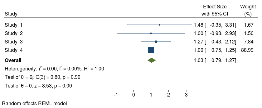
Forest plot without options studylabel() and eslabel()
syntax
Scenario II
Effect sizes computed from summary data
Binary summary data
(\(2\times 2\) tables)
Continuous summary data
(sample size, mean, and standard deviation for each group)
Hedges's \(g\), Cohen's \(d\), Glass's \(\Delta_1\) and \(\Delta_2\), and (raw) mean difference \(D\)
log odds-ratio \(\log\)(OR), \(\log\)(ORpeto), log risk-ratio \(\log\)(RR) , and risk difference \(RD\)
Effect sizes for binary data
. webuse bcg, clear
  (Efficacy of BCG vaccine against tuberculosis)
. keep studylbl npost - nnegc
. describe
------------------------------------------------------------------------------------------
storage display value
variable name type format label variable label
------------------------------------------------------------------------------------------
studylbl str27 %27s Study label
npost int %9.0g Number of TB positive cases in treated group
nnegt long %9.0g Number of TB negative cases in treated group
nposc int %9.0g Number of TB positive cases in control group
nnegc long %9.0g Number of TB negative cases in control group
------------------------------------------------------------------------------------------
| group | success | failure |
|---|---|---|
| treatment | npost = 4 | nnegt = 119 |
| control | nposc = 11 | nnegc = 128 |
each study, \(j\), yield a \(2\times 2\) table, e.g. for study 1:
     +--------------------------------------------------------+
     |               studylbl   npost   nnegt   nposc   nnegc |
     |--------------------------------------------------------|
  1. |          Aronson, 1948       4     119      11     128 |
  2. | Ferguson & Simes, 1949       6     300      29     274 |
  3. | Rosenthal et al., 1960       3     228      11     209 |
     +--------------------------------------------------------+
. list in 1/3their SEs and CIs
computes
meta esizeEffect sizes for binary data
. meta esize npost nnegt nposc nnegc Meta-analysis setting information
Study information
No. of studies: 13
Study label: Generic <--- controlled by studylabel()
Study size: _meta_studysize
Summary data: npost nnegt nposc nnegc
Effect size
Type: lnoratio <--- controlled by esize()
Label: Log Odds-Ratio <--- controlled by eslabel()
Variable: _meta_es
Zero-cells adj.: None; no zero cells <--- controlled by zerocells()
Precision
Std. Err.: _meta_se
CI: [_meta_cil, _meta_ciu]
CI level: 95% <--- controlled by level()
Model and method <--- controlled by random[()], fixed[()],
Model: Random-effects and common[()]
Method: REML
- Change the default (\(\log\)(OR)) effect size using option esize()
. meta esize npost nnegt nposc nnegc, esize(lnrratio) . meta update, esize(lnrratio) Or equivalently,
- Had there been zero cells, you may specify how to handle them via the zerocells() option
. meta update, zerocells(.2)

// or

. meta update, zerocells(tacc) - As is the case with meta set, you may specify which model to use via one of options random[()], fixed[()], or common[()] (default being random(reml))
. meta update, fixed(mhaenszel) studylabel(studylbl)- At any point in your analysis, you may use meta query to remind yourself of your current MA settings
. meta query -> meta esize n1 m1 sd1 n2 m2 sd2 , esize(cohensd) common
Meta-analysis setting information from meta esize
Study information
No. of studies: 10
Study label: Generic
Study size: _meta_studysize
Summary data: n1 m1 sd1 n2 m2 sd2
Effect size
Type: cohensd
Label: Cohen's d
Variable: _meta_es
Precision
Std. Err.: _meta_se
Std. Err. adj.: None
CI: [_meta_cil, _meta_ciu]
CI level: 95%
Model and method
Model: Common-effect
Method: Inverse-variance
syntax
local vs global options
. meta summarize in 1/3, common . meta summarize in 1/3, random(dlaird). meta summ in 1/3
In general, options specified with meta set and meta esize are defined globally throughout the entire MA
. meta esize n1 - sd2, random(ebayes) nometashow. meta summarize in 1/3
Meta-analysis summary                     Number of studies =      3
Random-effects model                      Heterogeneity:
Method: Empirical Bayes                               tau2 = 17.6396
                                                    I2 (%) =   77.89
                                                        H2 =    4.52

--------------------------------------------------------------------
            Study |     Hedges's g    [95% Conf. Interval]  % Weight
------------------+-------------------------------------------------
         Study  1 |        -22.020     -27.938     -16.101     28.60
         Study  2 |        -13.902     -17.554     -10.251     36.26
         Study  3 |        -12.906     -16.895      -8.917     35.14
------------------+-------------------------------------------------
            theta |        -15.874     -21.296     -10.452
--------------------------------------------------------------------
Test of theta = 0: z = -5.74                     Prob > |z| = 0.0000
Test of homogeneity: Q = chi2(2) = 6.81            Prob > Q = 0.0333
Meta-analysis summary                     Number of studies =      3
Common-effect model
Method: Inverse-variance

--------------------------------------------------------------------
            Study |     Hedges's g    [95% Conf. Interval]  % Weight
------------------+-------------------------------------------------
         Study  1 |        -22.020     -27.938     -16.101     17.16
         Study  2 |        -13.902     -17.554     -10.251     45.07
         Study  3 |        -12.906     -16.895      -8.917     37.77
------------------+-------------------------------------------------
            theta |        -14.919     -17.370     -12.467
--------------------------------------------------------------------
Test of theta = 0: z = -11.93                    Prob > |z| = 0.0000
Meta-analysis summary                     Number of studies =      3
Random-effects model                      Heterogeneity:
Method: DerSimonian-Laird                             tau2 = 12.0325
                                                    I2 (%) =   70.61
                                                        H2 =    3.40

--------------------------------------------------------------------
            Study |     Hedges's g    [95% Conf. Interval]  % Weight
------------------+-------------------------------------------------
         Study  1 |        -22.020     -27.938     -16.101     27.23
         Study  2 |        -13.902     -17.554     -10.251     37.15
         Study  3 |        -12.906     -16.895      -8.917     35.61
------------------+-------------------------------------------------
            theta |        -15.758     -20.462     -11.054
--------------------------------------------------------------------
Test of theta = 0: z = -6.57                     Prob > |z| = 0.0000
Test of homogeneity: Q = chi2(2) = 6.81            Prob > Q = 0.0333
Meta-analysis summary                     Number of studies =      3
Random-effects model                      Heterogeneity:
Method: Empirical Bayes                               tau2 = 17.6396
                                                    I2 (%) =   77.89
                                                        H2 =    4.52

--------------------------------------------------------------------
            Study |     Hedges's g    [95% Conf. Interval]  % Weight
------------------+-------------------------------------------------
         Study  1 |        -22.020     -27.938     -16.101     28.60
         Study  2 |        -13.902     -17.554     -10.251     36.26
         Study  3 |        -12.906     -16.895      -8.917     35.14
------------------+-------------------------------------------------
            theta |        -15.874     -21.296     -10.452
--------------------------------------------------------------------
Test of theta = 0: z = -5.74                     Prob > |z| = 0.0000
Test of homogeneity: Q = chi2(2) = 6.81            Prob > Q = 0.0333
local option
local option
global options
Further reading
- If you have access to summary data, use meta esize to compute and declare effect sizes such as an odds ratio or a Hedges’s \(g\).
- To check whether your data are already meta set or to see the current meta settings, use meta query
- To update some of your meta-analysis settings after the declaration, use meta update.
- Alternatively, if you have only precomputed (generic) effect sizes, use meta set.
Summary I
- If you specify CIs instead of SEs, the CIs must be symmetric (that is specify CIs for \(\log\)(OR), \(\log\)(RR), etc).
- meta set and meta esize create system variables with names starting with _meta_ to be used by all subsequent meta commands.
Data sets used
Two data sets will be used throughout this webinar, you may further explore them below
Exploring heterogenity
Meta-regression and subgroup-analysis
Case study: Efficacy of BCG vaccine against tuberculosis
- Heterogeneity: Variability among the effect sizes beyond what is expected due to random sampling (chance).
- Exploring the possible reasons for heterogeneity between studies is an important aspect of a MA
Quantifying heterogeneity
Sampling error
Between-study heterogeneity
Total observed heterogeneity
- meta regress focuses on explaining
(within-study heterogeneity)
meta summarize and meta forestplot report
What is meta-regression ?
- Meta-regression investigates whether between-study heterogeneity can be explained by one or more moderators
- Observations are the studies
- Two types of meta-regression:
- Fixed-effects (FE) meta-regression: assumes all heterogeneity is accounted for by the moderators
- Random-effects (RE) meta-regression: accounts for potential additional variability unexplained by the included moderators, also known as residual heterogeneity
- A weighted linear regression where:
- Outcome of interest (dependent variable) is the ES (_meta_es)
- Covariates (moderators) are recorded at the study level
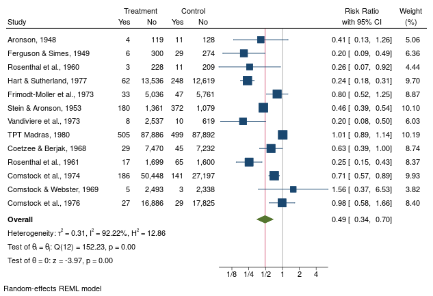
. webuse bcg, clear
  (Efficacy of BCG vaccine against tuberculosis)
. describe npost - studylbl
------------------------------------------------------------------------------------------
storage display value
variable name type format label variable label
------------------------------------------------------------------------------------------
npost int %9.0g Number of TB positive cases in treated group
nnegt long %9.0g Number of TB negative cases in treated group
nposc int %9.0g Number of TB positive cases in control group
nnegc long %9.0g Number of TB negative cases in control group
latitude byte %9.0g Absolute latitude of the study location (in
degrees)
alloc byte %10.0g alloc Method of treatment allocation
studylbl str27 %27s Study label
------------------------------------------------------------------------------------------
- MA consists of 13 studies (Colditz et al. [1994]) to evaluate the efficacy of the BCG vaccine against tuberculosis (TB)
- Vaccine efficacy has been controversial
+----------------------------------------------------------------------+
| author npost nnegt nposc nnegc latitude alloc |
|----------------------------------------------------------------------|
1. | Aronson 4 119 11 128 44 Random |
2. | Ferguson & Simes 6 300 29 274 55 Random |
3. | Rosenthal et al. 3 228 11 209 42 Random |
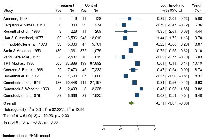
+----------------------------------------------------------------------+. list author npost - nnegc latitude alloc in 1/3. meta esize npost nnegt nposc nnegc, esize(lnrratio) studylabel(studylbl)
. meta forestplot
// create centered version of variable latitude
. summarize latitude, meanonly
. generate double latitude_c = latitude - r(mean)
. label variable latitude_c "Mean-centered latitude"
// Perform meta-regression
. meta regress latitude_c
. estat bubbleplot

. margins, at(latitude_c = (-18.5 -5.5 16.5))
- Then, some postestimation tools ...
Meta-regression
- Compute \(\log\)(RR) and declare MA settings (meta esize), summarize MA (meta forestplot), then perform meta-regression (meta regress)
What are we going to do ?
. meta esize npost - nnegc, esize(lnrratio) studylabel(studylbl)
. meta forestplot
. meta forest, eform nullrefline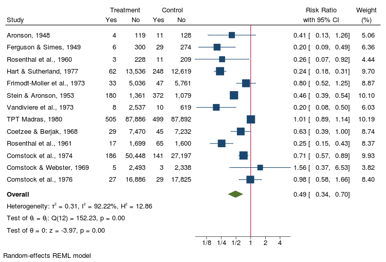
nonsignificant RR
nonoverlapping CIs
Berkey et al (1995) and Borenstein et al (2009) suggested that latitude (as a surrogate for climate) could explain some of the variation in the efficacy of the BCG vaccine
. meta regress latitude_c
Effect-size label:  Log Risk-Ratio
        Effect size:  _meta_es
          Std. Err.:  _meta_se

Random-effects meta-regression                      Number of obs  =        13
Method: REML                                        Residual heterogeneity:
                                                                tau2 =  .07635
                                                              I2 (%) =   68.39
                                                                  H2 =    3.16
                                                       R-squared (%) =   75.63
                                                    Wald chi2(1)   =     16.36
                                                    Prob > chi2    =    0.0001
------------------------------------------------------------------------------
    _meta_es |      Coef.   Std. Err.      z    P>|z|     [95% Conf. Interval]
-------------+----------------------------------------------------------------
  latitude_c |  -.0291017   .0071953    -4.04   0.000    -.0432043   -.0149991
       _cons |  -.7223204   .1076535    -6.71   0.000    -.9333174   -.5113234
------------------------------------------------------------------------------
Test of residual homogeneity: Q_res = chi2(11) = 30.73   Prob > Q_res = 0.0012
Implicitly, Y = \(\log\)(RR) stored in variable _meta_es
suppress via option nometashow
Quantifying heterogeneity
(within-study heterogeneity)
Sampling error
Between-study heterogeneity \(\tau^2_c\)
Total observed heterogeneity
\(\tau^2_c\) from
meta summarize
\(\tau^2\)
Explained by covariates
\(\tau^2\) from
meta regress
Postestimation tools
We may graph the relationship between the effect size and that moderator
. estat bubbleplot
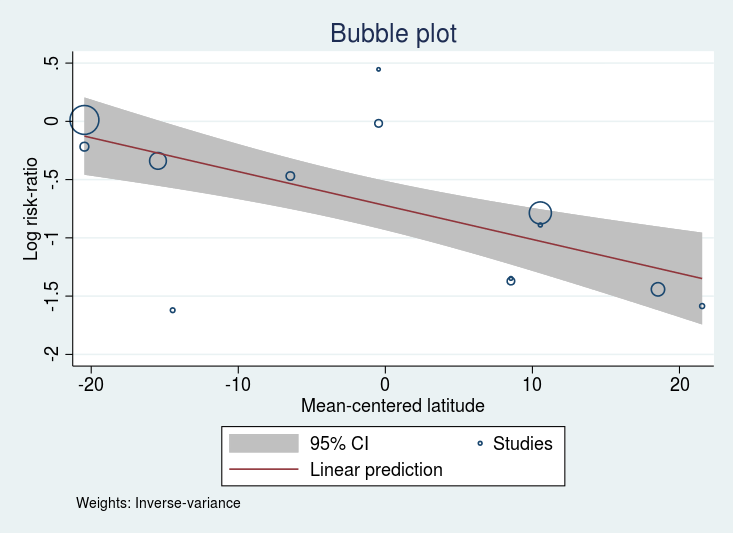
\(\log\)(RR) for the BCG vaccine declines as the distance from the equator increases
Ukraine
Nepal
Thailand
We can obtain estimates of the predicted \(\log\)(RR) at different latitudes using the margins command
. margins, at(latitude_c = (-18.5 -5.5 16.5))Adjusted predictions Number of obs = 13
Expression : Fitted values; fixed portion (xb), predict(fitted fixedonly)
1._at : latitude_c = -18.5
2._at : latitude_c = -5.5
3._at : latitude_c = 16.5
------------------------------------------------------------------------------
| Delta-method
| Margin Std. Err. z P>|z| [95% Conf. Interval]
-------------+----------------------------------------------------------------
_at |
1 | -.1839386 .1586092 -1.16 0.246 -.4948069 .1269297
2 | -.562261 .1091839 -5.15 0.000 -.7762574 -.3482645
3 | -1.202499 .1714274 -7.01 0.000 -1.53849 -.8665072
------------------------------------------------------------------------------
- The risk ratio for regions with latitude_c \(= 16.5\) (e.g. Ukraine) is \(\exp(-1.202499) = 0.3\), which means that the vaccine is expected to reduce the risk of TB by 70% for regions with that latitude
display these values on a forest plot
local col mcolor("maroon")
meta forest _id _esci _plot _weight latitude, nullrefline 	  	    ///
	columnopts(latitude, title("Latitude")) 			    ///
	customoverall(-.184 -.495  .127, label("{bf:latitude = 15}") `col') ///
	customoverall(-.562 -.776 -.348, label("{bf:latitude = 28}") `col') ///
	customoverall(-1.20 -1.54 -.867, label("{bf:latitude = 50}") `col') rr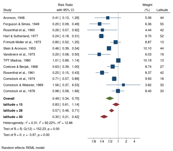
_id
_esci
_plot
_weight
- You may report your results as vaccine efficacies via the transform() option
meta forest _id _esci _plot _weight latitude, nullrefline 	  	    ///
	columnopts(latitude, title("Latitude")) 			    ///
	customoverall(-.184 -.495  .127, label("{bf:latitude = 15}") `col') ///
	customoverall(-.562 -.776 -.348, label("{bf:latitude = 28}") `col') ///
	customoverall(-1.20 -1.54 -.867, label("{bf:latitude = 50}") `col') ///
	transform("Vaccine efficacy": efficacy)
Other supported transformations within the transform() option are: corr, exp, invlogit, and tanh.
Further reading
Subgroup analysis
- Subgroup analysis involves dividing the data into subgroups, in order to make comparisons between them.
- The studies are grouped based on study or participants’ characteristics, and an overall effect-size estimate is computed for each group
- The goal of subgroup analysis is to compare these overall estimates across groups and determine whether the considered grouping helps explain some of the observed between-study heterogeneity.
- We will dichotomize latitude into two categories: hotter climate vs colder climate
. generate byte latitude_01 = latitude_c > 0

. label define latval 0 "hot climate" 1 "cold climate"

. label values latitude_01 latval
     +-------------------------------------------------------+
     |                    studylbl   latitude    latitude_01 |
     |-------------------------------------------------------|
  1. |               Aronson, 1948         44   cold climate |
  2. |      Ferguson & Simes, 1949         55   cold climate |
  3. |      Rosenthal et al., 1960         42   cold climate |
  4. |     Hart & Sutherland, 1977         52   cold climate |
  5. | Frimodt-Moller et al., 1973         13    hot climate |
     +-------------------------------------------------------+
. list studylbl latitude latitude_01 in 1/5
Compare the BCG vaccine efficacy in cold vs hot climate
. meta forestplot, subgroup(latitude_01) nullrefline transform(efficacy)
summary for each group
Test of \(H_0: \theta_{grp1} = \theta_{grp2}\)
Small-study effect (Publication bias)
- Small-study effects (Sterne, Gavaghan, and Egger 2000) is used in MA to describe the cases when the results of smaller studies differ systematically from the results of larger studies.
- One of the reasons behind small-study effect is publication bias (or more generally selection bias)
- Publication bias arises when the decision to publish a study depends on the statistical significance of its results.


Random subset
- Suppose that we are missing some of the studies in our MA.
Observed studies
valid conclusions albeit wider CIs, less powerful tests (less info)
systematically different
Studies not included in the MA (missing studies)
(e.g. when smaller studies with nonsignificant findings are suppressed from publication)
our meta-analytic results will be biased and decisions based on them are invalid
Tools for small-study effects analysis
- The funnel plot
- Tests for small-study effects
- The trim-and-fill analysis
- Simple funnel plot
- Contour-enhanced funnel plot (one-sided and two-sided significance contours)
- Several precision metrics
- Egger's, Peters's, and Harbord's regression-based tests with the possibility to include moderators to account for heterogeneity
- Begg and mazumdar's test
meta funnelplot
meta bias
meta trimfill
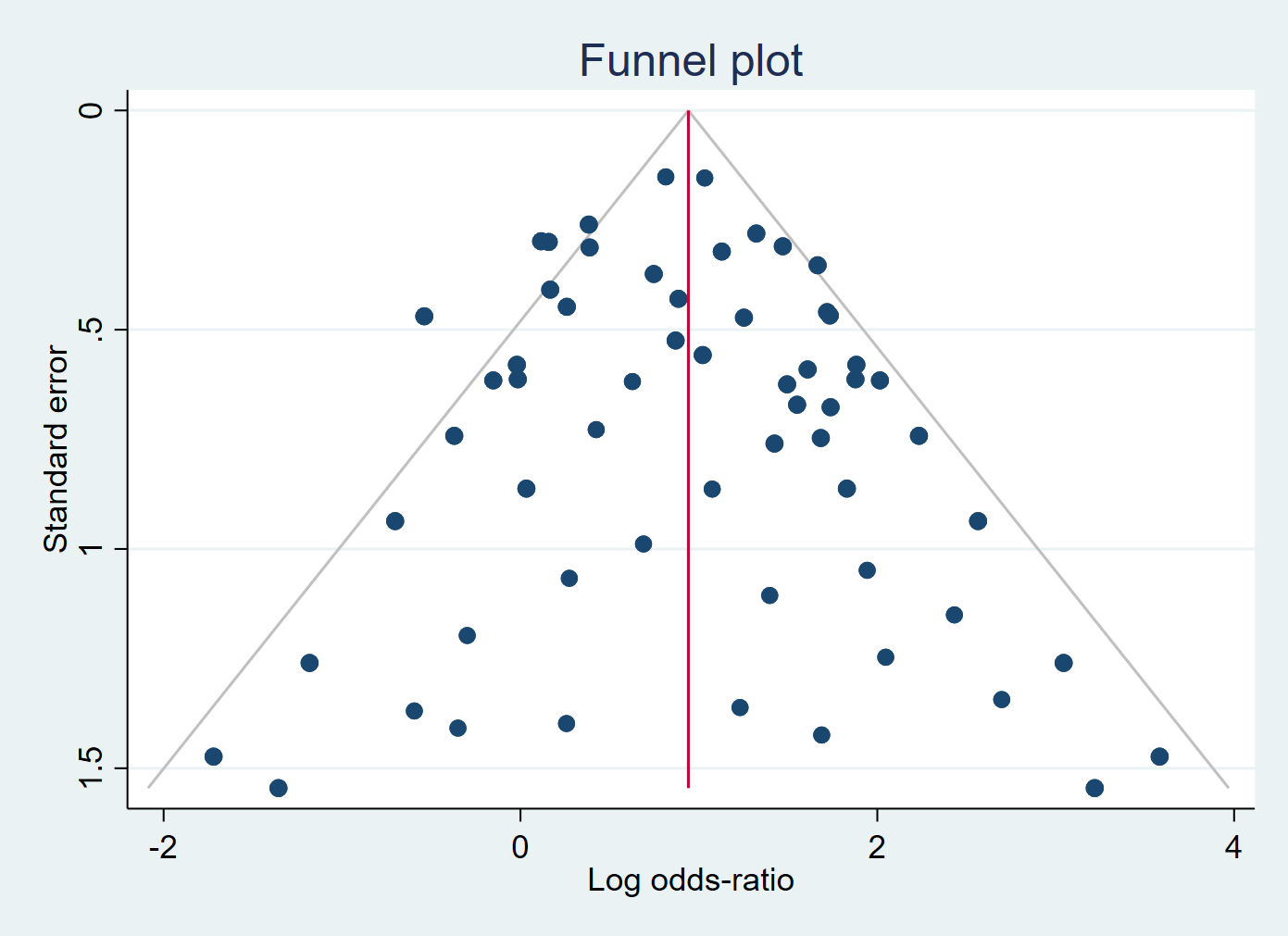

Small-study effect (potentially due to publication bias)
Little evidence of Small-study effect
which means the individual ES should be distributed randomly around the overall ES
Large and small studies tell the same story about \(\theta\)
Large and small studies tell different stories about \(\theta\)
. webuse nsaidsset, clear
 (Effectiveness of nonsteroidal anti-inflammatory drugs; set with -meta esize-)
. meta funnelplot
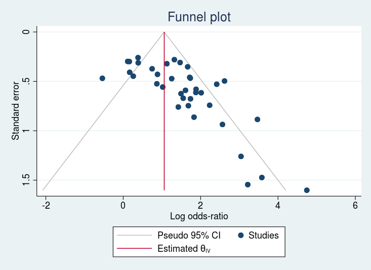
 Effect-size label:  Log Odds-Ratio
        Effect size:  _meta_es
          Std. Err.:  _meta_se
              Model:  Common-effect
             Method:  Inverse-variance
gap (missing studies ?)
. meta funnelplot, contours(1 5 10)
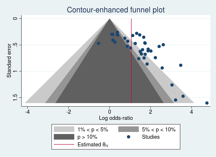
. meta funnelplot, contours(1 5 10) metric(invvar)

- You may enhance the contour funnel plot via the addplot() option
. scalar theta = r(theta) // obtained from previous -meta funnel- command r() results

// position legend at 10 o'clock inside the graph region
. local legopts ring(0) position(10) cols(1) size(small) symxsize(*0.6)

. local opts horizontal range(0 1.6) lpattern(dash) lcolor("red") ///
	legend(order(1 2 3 4 5 6) label(6 "95% pseudo CI") `legopts')

. meta funnel, contours(1 5 10) ///
      addplot(function theta-1.96*x, `opts' || function theta+1.96*x, `opts')
. meta bias, harbord - We will test for funnel-plot asymmetry and use the Harbord's test instead of the Egger's test as we are working with \(\log\)(OR)
 Effect-size label:  Log Odds-Ratio
        Effect size:  _meta_es
          Std. Err.:  _meta_se

Regression-based Harbord test for small-study effects
Random-effects model
Method: REML

H0: beta1 = 0; no small-study effects
            beta1 =      3.03
      SE of beta1 =     0.741
                z =      4.09
       Prob > |z| =    0.0000
Nonparametric trim-and-fill analysis of publication bias
Linear estimator, imputing on the left

Iteration                            Number of studies =     47
  Model: Random-effects                       observed =     37
 Method: REML                                  imputed =     10

Pooling
  Model: Random-effects
 Method: REML

---------------------------------------------------------------
             Studies |   Log Odds-Ratio    [95% Conf. Interval]
---------------------+-----------------------------------------
            Observed |            1.322       1.031       1.613
  Observed + Imputed |            1.035       0.726       1.343
---------------------------------------------------------------
. meta trimfill, funnel(contours(1 5 10) legend(`legopts'))- We can perform a trim-and-fill analysis to assess the effect of missing studies on the overall ES and request a contour-enhanced funnel plot based on the complete (observed + filled) set studies

Summary III
- Publication bias occurs if studies with favourable results are more likely to be published than studies with unfavourable results.
- Small-study effect is manifested graphically by funnel-plot asymmetry
- Publication bias is only one of the reasons behind funnel-plot asymmetry.
- Publication bias should be assessed after you have accounted for heterogeneity in your MA
- You can investigate small-study effects visually via meta funnelplot, test for it via meta bias, and assess its impact on the overall ES via meta trimfill
Other features
- Cumulative MA forest plots
- L'Abbé plots
- Multiple subgroup analyses forest plots
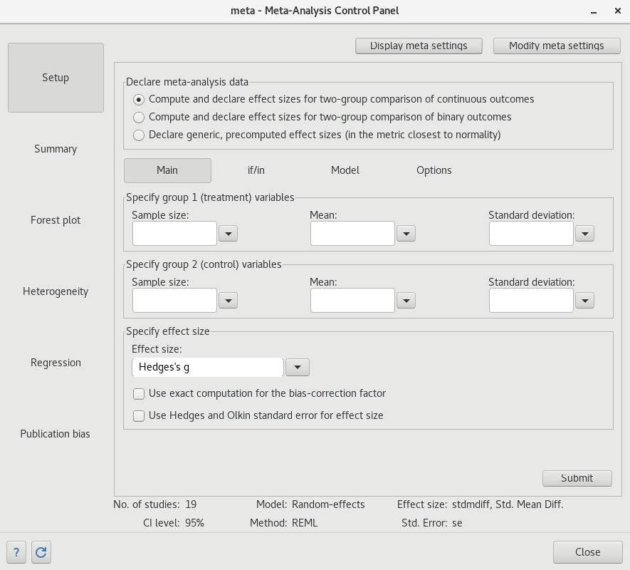
The meta control panel
Prefer to avoid typing commands ? Everything I have showed you can be done in the meta control panel with few mouse clicks

meta set
meta esize
meta summarize
meta forestplot
meta labbeplot
meta regress
estat bubbleplot
meta funnelplot
meta bias
meta trimfillA tour of the meta control panel
Summary
- Effect sizes for binary and continuous data may be computed via meta esize and generic (pre-computed) ES may be specified via meta set
- It is important to include an assessment of publication bias to insure the integrity of the MA . This may be done using the meta funnelplot, meta bias and meta trimfill commands
- When substantial heterogeneity is present among the studies, the reasons behind this heterogeneity should be explored via meta-regression ( meta regress) or subgroup analysis ( meta summarize, subgroup())
- Use meta update and meta query to update and describe your current MA settings, respectively
- Results of a MA are best summarized numerically using meta summarize, or graphically using meta forestplot. This includes subgroup-analysis forest plots and CMA forest plots.