Example 3: Work with multiple datasets (frames)
Stata 16 introduced frames, allowing you to simultaneously work with multiple datasets in memory. To learn more about frames, see the [D] frames intro in the Stata Data Management Reference Manual. In this example, we illustrate how to pass data and results between Python and Stata’s frames.
First, we load the Iris dataset in Stata. This dataset was used in Fisher’s (1936) article and originally collected by Anderson (1935). The data consist of four features measured on 50 samples from each of three Iris species. The four features are the length and width of the sepal and petal. The three species are Iris setosa, Iris versicolor, and Iris virginica.
[13]:
%%stata
use http://www.stata-press.com/data/r18/iris, clear
describe
label list species
. use http://www.stata-press.com/data/r18/iris, clear
(Iris data)

. describe

Contains data from http://www.stata-press.com/data/r18/iris.dta
 Observations:           150                  Iris data
    Variables:             5                  18 Jan 2022 13:23
                                              (_dta has notes)
-------------------------------------------------------------------------------
Variable      Storage   Display    Value
    name         type    format    label      Variable label
-------------------------------------------------------------------------------
iris            byte    %10.0g     species    Iris species
seplen          double  %4.1f                 Sepal length in cm
sepwid          double  %4.1f                 Sepal width in cm
petlen          double  %4.1f                 Petal length in cm
petwid          double  %4.1f                 Petal width in cm
-------------------------------------------------------------------------------
Sorted by:

. label list species
species:
           1 Setosa
           2 Versicolor
           3 Virginica

.
Our goal is to build a classifier using those four features to detect the iris type. We will use the Support Vector Machine (SVM) classifier within the scikit-learn Python package to achieve this goal. First, we split the data into the training and test datasets, and we store the datasets in the training and test frames in Stata. The training dataset contains 80% of the observations and the test dataset contains 20% of the observations. Then, we store the two frames into Python as NumPy arrays with the same names.
[14]:
%%stata -fouta training,test
// split the original dataset into training and test
// datasets, which contain 80% and 20% of the observations, respectively
splitsample, generate(svar, replace) split(0.8 0.2) show rseed(16)

// create a new frame to hold each dataset
frame put iris seplen sepwid petlen petwid if svar==1, into(training)
frame put iris seplen sepwid petlen petwid if svar==2, into(test)
. // split the original dataset into training and test
. // datasets, which contain 80% and 20% of the observations, respectively
. splitsample, generate(svar, replace) split(0.8 0.2) show rseed(16)

       svar |      Freq.     Percent        Cum.
------------+-----------------------------------
          1 |        120       80.00       80.00
          2 |         30       20.00      100.00
------------+-----------------------------------
      Total |        150      100.00

.
. // create a new frame to hold each dataset
. frame put iris seplen sepwid petlen petwid if svar==1, into(training)

. frame put iris seplen sepwid petlen petwid if svar==2, into(test)

.
Now we have two NumPy arrays in Python, training and test. Below, we split each array into two sub-arrays to store the features and labels separately.
[15]:
X_train = training[:, 1:]
y_train = training[:, 0]
X_test = test[:, 1:]
y_test = test[:, 0]
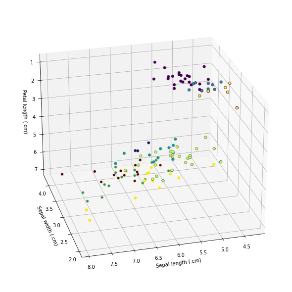
Next, we use the Matplotlib package in Python to create a 3D plot using the sepal length, sepal width, and petal length from the training dataset.
[16]:
import matplotlib.pyplot as plt
from mpl_toolkits.mplot3d import Axes3D
[17]:
%matplotlib inline

fig = plt.figure(1, figsize=(10, 8))
ax = Axes3D(fig, elev=-155, azim=105)
ax.scatter(X_train[:, 0], X_train[:, 1], X_train[:, 2], c=y_train, s=30)
ax.set_xlabel("Sepal length (.cm)")
ax.set_ylabel("Sepal width (.cm)")
ax.set_zlabel("Petal length (.cm)")
plt.show()
Then, we use X_train and y_train to train the SVM classification model.
[18]:
from sklearn.svm import SVC

svc_clf = SVC(gamma='auto', probability=True, random_state=17)
svc_clf.fit(X_train, y_train)
[18]:
SVC(C=1.0, break_ties=False, cache_size=200, class_weight=None, coef0=0.0,
    decision_function_shape='ovr', degree=3, gamma='auto', kernel='rbf',
    max_iter=-1, probability=True, random_state=17, shrinking=True, tol=0.001,
    verbose=False)
Next, we use X_test and y_test to evaluate the performance of the training model. We also predict the species type of each flower and the probabilities that it belongs to the three species in the test dataset.
[19]:
from sklearn import metrics

y_pred = svc_clf.predict(X_test)
y_pred_prob = svc_clf.predict_proba(X_test)
print(metrics.accuracy_score(y_test, y_pred))
0.9
Comparing the predicted species types with the true types, we find that 90% of the flowers are correctly classified.
Below, we use the Frame class within the Stata Function Interface (sfi) module to store our results from Python into the test frame in Stata. We store the predicted species types from the array y_pred in a new byte variable, irispr. And we create three float variables to store the probabilities that the flowers belong to each of the three species types from the array y_pred_prob.
[20]:
from sfi import Frame

# connect to the test frame within Stata
fr = Frame.connect('test')
fr.addVarByte('irispr')
fr.addVarFloat('pr1')
fr.addVarFloat('pr2')
fr.addVarFloat('pr3')

fr.store('irispr', None, y_pred)
fr.store('pr1 pr2 pr3', None, y_pred_prob)
In Stata, we change the current working frame to test. We attach the value label species to irispr, and we use the tabulate command to display a classification table.
[21]:
%%stata
// change the current working frame to test
frame change test

// label the variable
label values irispr species
label variable irispr predicted

// display the classification table
tabulate iris irispr, row
. // change the current working frame to test
. frame change test

.
. // label the variable
. label values irispr species

. label variable irispr predicted

.
. // display the classification table
. tabulate iris irispr, row

+----------------+
| Key            |
|----------------|
|   frequency    |
| row percentage |
+----------------+

      Iris |            predicted
   species |    Setosa  Versicolo  Virginica |     Total
-----------+---------------------------------+----------
    Setosa |        11          0          0 |        11
           |    100.00       0.00       0.00 |    100.00
-----------+---------------------------------+----------
Versicolor |         0          9          3 |        12
           |      0.00      75.00      25.00 |    100.00
-----------+---------------------------------+----------
 Virginica |         0          0          7 |         7
           |      0.00       0.00     100.00 |    100.00
-----------+---------------------------------+----------
     Total |        11          9         10 |        30
           |     36.67      30.00      33.33 |    100.00

.
We also list the first three observations of the test frame to view the predicted species types, and we list flowers that have been misclassified.
[22]:
%%stata
// list the first 3 observations
list in 1/3

// list flowers that have been misclassified
list iris irispr pr1 pr2 pr3 if iris!=irispr
. // list the first 3 observations
. list in 1/3

     +----------------------------------------------------------------+
  1. |   iris | seplen | sepwid | petlen | petwid | irispr |      pr1 |
     | Setosa |    4.9 |    3.0 |    1.4 |    0.2 | Setosa | .9644561 |
     |----------------------------------------------------------------|
     |                pr2            |                 pr3            |
     |            .017525            |            .0180189            |
     +----------------------------------------------------------------+

     +----------------------------------------------------------------+
  2. |   iris | seplen | sepwid | petlen | petwid | irispr |      pr1 |
     | Setosa |    5.4 |    3.9 |    1.7 |    0.4 | Setosa | .9430715 |
     |----------------------------------------------------------------|
     |                pr2            |                 pr3            |
     |           .0315332            |            .0253953            |
     +----------------------------------------------------------------+

     +----------------------------------------------------------------+
  3. |   iris | seplen | sepwid | petlen | petwid | irispr |      pr1 |
     | Setosa |    5.0 |    3.4 |    1.5 |    0.2 | Setosa |  .964682 |
     |----------------------------------------------------------------|
     |                pr2            |                 pr3            |
     |           .0175306            |            .0177874            |
     +----------------------------------------------------------------+

.
. // list flowers that have been misclassified
. list iris irispr pr1 pr2 pr3 if iris!=irispr

     +---------------------------------------------------------+
     |       iris      irispr        pr1        pr2        pr3 |
     |---------------------------------------------------------|
 16. | Versicolor   Virginica   .0140703   .3429256   .6430042 |
 18. | Versicolor   Virginica   .0146823   .3348792   .6504385 |
 19. | Versicolor   Virginica   .0113467   .1247777   .8638756 |
     +---------------------------------------------------------+

.