Spatial autoregression is a regression model that takes into account of spatial spillover effects.
Spatial spillover defines how “Where you are matters to yourself and to others”.
First, we need to understand what is no spatial spillover. Let us consider a simple linear regression model without any spatial interactions.
$$ \begin{equation} hrate_i = \beta_0 + \beta_1*unemployment_{i} + \epsilon_i \label{eq:nosp} \end{equation} $$
No spillover means
For
. clear all

. copy http://www.stata-press.com/data/r15/homicide1990.dta ., replace

. copy http://www.stata-press.com/data/r15/homicide1990_shp.dta ., replace

. use homicide1990
(S.Messner et al.(2000), U.S southern county homicide rates in 1990)

. keep if sname == "Texas"
(1,158 observations deleted)

. spregress hrate unemployment, gs2sls
  (254 observations)
  (254 observations (places) used)

Spatial autoregressive model                    Number of obs     =        254
GS2SLS estimates                                Wald chi2(1)      =      10.96
                                                Prob > chi2       =     0.0009
                                                Pseudo R2         =     0.0414

------------------------------------------------------------------------------
       hrate |      Coef.   Std. Err.      z    P>|z|     [95% Conf. Interval]
-------------+----------------------------------------------------------------
unemployment |   .5007108   .1512161     3.31   0.001     .2043328    .7970888
       _cons |   4.894674    1.12093     4.37   0.000     2.697691    7.091656
------------------------------------------------------------------------------
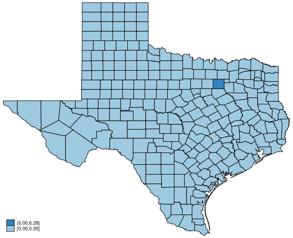
Here we show there is no spillover. We can do this in
. preserve

.
. /*
>         Step 1 : Predict hrate using the original data
> */
. predict y0
(option rform assumed; reduced-form mean)

.
. /*
>         Step 2 : Change *unemployment* in __Dallas__ and predict *hrate* agai
> n
> */
. replace unemployment = 20 if cname == "Dallas"
(1 real change made)

. predict y1
(option rform assumed; reduced-form mean)

.
. /*
>         Step 3 : Compute the difference between these two predictions
> */
. generate y_diff = y1 - y0

. grmap y_diff, clmethod(unique) fcolor(Blues) title("No spillover")

. restore

We now explicitly let $y_i$ depends on $x_j$. For example, we now allows hrate in one county depends on the unemployment in its neighborhood.
We use a contiguity matrix $W$. (Later, we will talk more about spatial weighting matrix here)
$$ \begin{equation} hrate_i = \beta_0 + \beta_1*unemployment_{i} + \gamma_1\sum_{j=1}^N W_{i,j}*unemployment_{j} + \epsilon_i \end{equation} $$
Local spillover means
. /*
>         Step 1. create a contiguity spatial weighting matrix W based
> */
. spmatrix create contiguity W

. /*
>         Step 2.
> */
. spregress hrate unemployment, ivarlag(W: unemployment) gs2sls
  (254 observations)
  (254 observations (places) used)
  (weighting matrix defines 254 places)

Spatial autoregressive model                    Number of obs     =        254
GS2SLS estimates                                Wald chi2(2)      =      11.77
                                                Prob > chi2       =     0.0028
                                                Pseudo R2         =     0.0443

------------------------------------------------------------------------------
       hrate |      Coef.   Std. Err.      z    P>|z|     [95% Conf. Interval]
-------------+----------------------------------------------------------------
hrate        |
unemployment |   .4533321   .1602732     2.83   0.005     .1392023    .7674619
       _cons |   3.976553   1.529133     2.60   0.009     .9795067      6.9736
-------------+----------------------------------------------------------------
W            |
unemployment |   .2126063   .2412739     0.88   0.378    -.2602818    .6854945
------------------------------------------------------------------------------
Wald test of spatial terms:          chi2(1) = 0.78       Prob > chi2 = 0.3782
As in the no spillover case, we can show the local spillover in the exactly same 3 steps.
. preserve

. predict y0
(option rform assumed; reduced-form mean)

. replace unemployment = 20 if cname == "Dallas"
(1 real change made)

. predict y1
(option rform assumed; reduced-form mean)

. generate y_diff = y1 - y0

. grmap y_diff, fcolor(Blues) clmethod(unique)    ///
>         title("Local spillover")

. restore

Global spillover means one change in one location will potentially affect outcomes everywhere. For example, we allow homicide rate in one county depends on homicide rate in its neighbors.
$$ \begin{equation} hrate_i = \beta_0 + \beta_1*unemployment_{i} + \lambda_1\sum_{j=1}^N W_{i,j}*hrate_{j} + \epsilon_i \end{equation} $$
Global spillover means
. spregress hrate unemployment, dvarlag(W) gs2sls
  (254 observations)
  (254 observations (places) used)
  (weighting matrix defines 254 places)

Spatial autoregressive model                    Number of obs     =        254
GS2SLS estimates                                Wald chi2(2)      =      14.23
                                                Prob > chi2       =     0.0008
                                                Pseudo R2         =     0.0424

------------------------------------------------------------------------------
       hrate |      Coef.   Std. Err.      z    P>|z|     [95% Conf. Interval]
-------------+----------------------------------------------------------------
hrate        |
unemployment |   .4584241    .152503     3.01   0.003     .1595237    .7573245
       _cons |   2.720913   1.653105     1.65   0.100    -.5191143    5.960939
-------------+----------------------------------------------------------------
W            |
       hrate |   .3414964   .1914865     1.78   0.075    -.0338103    .7168031
------------------------------------------------------------------------------
Wald test of spatial terms:          chi2(1) = 3.18       Prob > chi2 = 0.0745
We repeat the 3 steps.
. preserve

. predict y0
(option rform assumed; reduced-form mean)

. replace unemployment = 20 if cname == "Dallas"
(1 real change made)

. predict y1
(option rform assumed; reduced-form mean)

. generate y_diff = y1 - y0

. grmap y_diff, clnumber(6) title("Global spillover")

. restore

The magic comes from the term $\lambda W y$.
The model is $$ \begin{align} y &= X\beta + \lambda W y + \epsilon \\ E(y|X) &= (I - \lambda W)^{-1} X\beta \end{align} $$
So if we change $x$ in observation $i$, the predicted outcome change is $$ \begin{align} E(y|X_1) - E(y|X_0) &= (I - \lambda W)^{-1} \Delta X \beta \nonumber \\ &= (I + \lambda W + \lambda^2 W^2 + \lambda^3 W^3 + \ldots) \Delta X \beta \end{align} $$
After fitting the model, we usually need to use estat impact compute the direct, indirect, and total impacts summary statistics and their standard errors. For example,
. estat impact

progress   :100%

Average impacts                                 Number of obs     =        254

------------------------------------------------------------------------------
             |            Delta-Method
             |      dy/dx   Std. Err.      z    P>|z|     [95% Conf. Interval]
-------------+----------------------------------------------------------------
direct       |
unemployment |   .4666538   .1539861     3.03   0.002     .1648466    .7684609
-------------+----------------------------------------------------------------
indirect     |
unemployment |   .1910068   .1565581     1.22   0.222    -.1158414     .497855
-------------+----------------------------------------------------------------
total        |
unemployment |   .6576605   .2519366     2.61   0.009     .1638739    1.151447
------------------------------------------------------------------------------
Question : where do these numbers come from ? See answers.
Remember that both outcome and covariate are vectors
$$ \begin{align} \frac{\partial y}{\partial x} = \begin{bmatrix} \color{red}\frac{\partial y_1}{\partial x_1} & \ldots & \ldots & \ldots & \frac{\partial y_1}{\partial x_n} \\ \vdots & \color{red}\ddots & & & \vdots \\ \frac{\partial y_k}{\partial x_1} & \ldots & \color{red}\frac{\partial y_k}{\partial x_k} & \ldots & \frac{\partial y_k}{\partial x_n} \\ \vdots & & & \color{red}\ddots & \vdots \\ \frac{\partial y_n}{\partial x_1} & \ldots & \ldots & \ldots & \color{red}\frac{\partial y_n}{\partial x_n} \end{bmatrix} \label{eq:dydx} \end{align} $$
$$ \begin{align} \text{Direct impacts} &= \begin{bmatrix} \color{red}\frac{\partial y_1}{\partial x_1} & & & & \\ & \color{red}\ddots & & & \\ & & \color{red}\frac{\partial y_k}{\partial x_k} & & \\ & & & \color{red}\ddots & \\ & & & & \color{red}\frac{\partial y_n}{\partial x_n} \end{bmatrix} \label{eq:direct} \end{align} $$
$$ \begin{align} \text{ADI} & = \frac{1}{n} \sum_{i=1}^n \frac{\partial y_i}{\partial x_i} \end{align} $$
$$ \begin{align*} \begin{bmatrix} \color{red}\frac{\partial y_1}{\partial x_1} & \ldots & \ldots & \ldots & \frac{\partial y_1}{\partial x_n} \\ \vdots & \color{red}\ddots & & & \vdots \\ \frac{\partial y_k}{\partial x_1} & \ldots & \color{red}\frac{\partial y_k}{\partial x_k} & \ldots & \frac{\partial y_k}{\partial x_n} \\ \vdots & & & \color{red}\ddots & \vdots \\ \frac{\partial y_n}{\partial x_1} & \ldots & \ldots & \ldots & \color{red}\frac{\partial y_n}{\partial x_n} \end{bmatrix} &= \begin{bmatrix} \color{red}\frac{\partial y_1}{\partial x_1} & & & & \\ & \color{red}\ddots & & & \\ & & \color{red}\frac{\partial y_k}{\partial x_k} & & \\ & & & \color{red}\ddots & \\ & & & & \color{red}\frac{\partial y_n}{\partial x_n} \end{bmatrix} + \begin{bmatrix} \color{red}0 & \ldots & \ldots & \ldots & \frac{\partial y_1}{\partial x_n} \\ \vdots & \color{red}\ddots & & & \vdots \\ \frac{\partial y_k}{\partial x_1} & \ldots & \color{red}0 & \ldots & \frac{\partial y_k}{\partial x_n} \\ \vdots & & & \color{red}\ddots & \vdots \\ \frac{\partial y_n}{\partial x_1} & \ldots & \ldots & \ldots & \color{red}0 \end{bmatrix} \\ \\ \text{Total impacts} &= \text{direct impacts} + \text{indirect impacts} \end{align*} $$
$$ \begin{align} \text{ATI} &= \frac{1}{n} \sum_{i=1}^n \sum_{j=1}^n \frac{\partial y_i}{\partial x_j} \end{align} $$
In a normal linear regression, the coefficients itself tell us exactly how would outcome $y$ change when there is change in covariates $x$. Actually, the indirect impacts are always zero in this case.
However, in spatial autoregression, the impacts of change in $x$ to the outcome $y$ is spatially spread out. It is a very complex process, and just the coefficients itself CANNOT describe this impact change in $y$. We need estat impact to quantify the spatial spillover effects.