What's this about?

Sometimes, processes evolve over time with discrete changes in outcomes.

Think of economic recessions and expansions. At the onset of a recession, output and employment fall and stay low, and then, later, output and employment increase. Think of bipolar disorders in which there are manic periods followed by depressive periods, and the process repeats. Statistically, means, variances, and other parameters are changing across episodes (regimes). Our problem is to estimate when regimes change and the values of the parameters associated with each regime. Asking when regimes change is equivalent to asking how long regimes persist.

In Markov-transition models, in addition to estimating the means, variances, etc. of each regime, we estimate the probability of regime change as well. The estimated transition probabilities for some problem might be, the following:

    
from/to
state
   1          2   

   1  
   0.82      0.18   
   2  
   0.75      0.25   

Start in state 1. The probability of transiting from state 1 to state 1 is 0.82. Said differently, once in state 1, the process tends to stay there. With probability 0.18, however, the process transits to state 2. State 2 is not as persistent. With probability 0.75, the processes revert from state 2 to state 1 in the next time period.

Markov-switching models are not limited to two regimes, although two-regime models are common.

In the example above, we described the switching as being abrupt; the probability instantly changed. Such Markov models are called dynamic models. Markov models can also accommodate smoother changes by modeling the transition probabilities as an autoregressive process.

Thus switching can be smooth or abrupt.

Let's see it work

Let's look at mean changes across regimes. In particular, we will analyze the Federal Funds Rate. The Federal Funds Rate is the interest rate that the central bank of the U.S. charges commercial banks for overnight loans. We are going to look at changes in the federal funds rate from 1954 to the end of 2010. Here are the data:

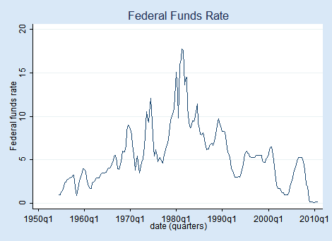
We have quarterly data. High interest rates seem to characterize the seventies and eighties. We will assume there is another regime for lower interest rates that seem to characterize the other decades.

To fit a dynamic-switching (abrupt-change) model with two regimes, we type

. mswitch dr fedfunds

Performing EM optimizaiton:

Performing gradient-based optimization:


Iteration 0:
   log likelihood = -508.66031
Iteration 1:
   log likelihood =  -508.6382
Iteration 2:
   log likelihood = -508.63592
Iteration 3:
   log likelihood = -508.63592

Markov-switching dynamic regression

Sample: 1954q3 - 2010q4                        No. of obs        =        226
Number of states =    2                        AIC               =     4,5455
Unconditional probabilities: transition        HQIC              =     4,5760
                                               SBIC              =     4,6211
Log likelihood = -508.63592

    fedfunds 
      Coef.   Std. Err.      z    P>|z|     [95% Conf. Interval]

State1       

       _cons 
    3.70877   .1767083    20.99   0.000     3.362428    4.055112

State2

       _cons 
   9.556793   .2999889    31.86   0.000     8.968826    10.14476

       sigma 
   2.107562   .1008692                      1.918851    2.314831

         p11 
   .9820939   .0104002                      .9450805    .9943119

         p21 
   .0503587   .0268434                      .0173432    .1374344

Reported in the output above are

• the means of the two states (_cons);
• a single standard deviation for the entire process (sigma); and
• the transition probabilities for state 1 to 1 and state 2 to 1 (p11 and p21).

State1 is the moderate-rate state (mean of 3.71%).

State2 is the high-rate state (mean 9.56%).

from/to
state
   1          2   

   1  
   0.98   1 - 0.98 
   2  
   0.05   1 - 0.05 

Both states are incredibly persistent (1->1 and 2->2 probabilities of 0.98 and 0.95).

Among the things you can predict after estimation is the probability of being in the various states. We have only two states, and thus the probability of being in (say) state 2 tells us the probability for both states. We can obtain the predicted probability and graph it along with the original data:

. predict prfed, pr

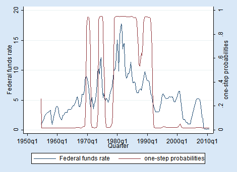
The model has little uncertainty as to regime at every point in time. We see three periods of high-rate states and four periods of moderate-rate states.

Let's see it work

Let's look at an example of disease outbreak, namely mumps per 10,000 residents in New York City between 1929 and 1972. You might think that outbreaks correspond to mean changes, but what we see in the data is an even greater change in variance:

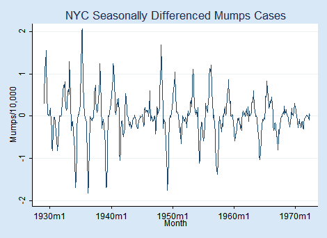
We graphed variable S12.mumpspc, meaning seasonally differenced mumps cases per capita over a 12-month period, and we are going to analyze S12.mumpspc.

We are going to assume two regimes in which the mean and variance of S12.mumpspc change. To fit a dynamic (abrupt-change) model, we type

. mswitch dr S12.mumpspc, varswitch switch(LS12.mumpspc, noconstant)

Performing EM optimizaiton:

Performing gradient-based optimization:


Iteration 0:
   log likelihood =   110.9372  (not concave)
Iteration 1:
   log likelihood =  120.68028  
Iteration 2:
   log likelihood =  123.23244  
Iteration 3:
   log likelihood =  131.47084  
Iteration 3:
   log likelihood =  131.72182  
Iteration 3:
   log likelihood =   131.7225  
Iteration 3:
   log likelihood =   131.7225  

Markov-switching dynamic regression

Sample: 1929m2 - 1972m6                        No. of obs        =        521
Number of states =    2                        AIC               =    -0.4826
Unconditional probabilities: transition        HQIC              =    -0.4634
                                               SBIC              =    -0.4336
Log likelihood = 131.7225

 S12.mumspc 
      Coef.   Std. Err.      z    P>|z|     [95% Conf. Interval]

State1       

     mumpspc 

       LS12. 
   .4202751   .0167461    25.10   0.000     .3874533    .4530968

State2       

     mumpspc 

       LS12. 
   .9847369   .0258383    38.11   0.000     .9340947    1.035379

      sigma1 
   .0562405   .0050954                      .0470901     .067169

      sigma2 
   .2611362   .0111191                      .2402278    .2838644

         p11 
    .762733   .0362619                      .6846007    .8264175

         p12 
   .1473767   .0257599                      .1036675     .205294

Reported are

• the means of the two states of S12.mumpspc (0.42 and 0.98);
• the standard deviations of the two states (0.06 and 0.26); and
• the transition probabilities for state 1 to 1 and state 2 to 1 (0.76 and 0.15).

State 1 is the low-variance state.

The full set of transition probabilities is the following:

from/to
state
   1          2   

   1  
   0.76   1 - 0.76 
   2  
   0.15   1 - 0.15 

As in the previous model, the states are persistent.

mswitch has other features such as calculating smoother transitions using autoregressive models.

Tell me more

You can see even more worked examples, read the full syntax of mswitch, learn about autoregressive models, and more in the documentation for mswitch; see [TS] mswitch.

Read the overview from the Stata News.